Rolling Correlations and Applications for Traders and Investors1. Introduction
Markets are dynamic, and the relationships between assets are constantly shifting. Static correlation values, calculated over fixed periods, may fail to capture these changes, leading traders to miss critical insights. Rolling correlations, on the other hand, provide a continuous view of how correlations evolve over time, making them a powerful tool for dynamic market analysis.
This article explores the concept of rolling correlations, illustrates key trends with examples like ZN (10-Year Treasuries), GC (Gold Futures), and 6J (Japanese Yen Futures), and discusses their practical applications for portfolio diversification, risk management, and timing market entries and exits.
2. Understanding Rolling Correlations
o What Are Rolling Correlations?
Rolling correlations measure the relationship between two assets over a moving window of time. By recalculating correlations at each step, traders can observe how asset relationships strengthen, weaken, or even reverse.
For example, the rolling correlation between ZN and GC reveals periods of alignment (strong correlation) during economic uncertainty and divergence when driven by differing macro forces.
o Why Rolling Correlations Matter:
Capture dynamic changes in market relationships.
Detect regime shifts, such as transitions from risk-on to risk-off sentiment.
Provide context for recent price movements and their alignment with historical trends.
o Impact of Window Length: The length of the rolling window (e.g., 63 days for daily, 26 weeks for weekly) impacts the sensitivity of correlations:
Shorter Windows: Capture rapid changes but may introduce noise.
Longer Windows: Smooth out fluctuations, focusing on sustained trends.
3. Case Study: ZN (Treasuries) vs GC (Gold Futures)
Examining the rolling correlation between ZN and GC reveals valuable insights into their behavior as safe-haven assets:
o Daily Rolling Correlation:
High variability reflects the influence of short-term market drivers like inflation data or central bank announcements.
Peaks in correlation align with periods of heightened risk aversion, such as in early 2020 during the onset of the COVID-19 pandemic.
o Weekly Rolling Correlation:
Provides a clearer view of their shared response to macroeconomic conditions.
For example, the correlation strengthens during sustained inflationary periods when both assets are sought as hedges.
o Monthly Rolling Correlation:
Reflects structural trends, such as prolonged periods of monetary easing or tightening.
Divergences, such as during mid-2023, may indicate unique demand drivers for each asset.
These observations highlight how rolling correlations help traders understand the evolving relationship between key assets and their implications for broader market trends.
4. Applications of Rolling Correlations
Rolling correlations are more than just an analytical tool; they offer practical applications for traders and investors:
1. Portfolio Diversification:
By monitoring rolling correlations, traders can identify periods when traditionally uncorrelated assets start aligning, reducing diversification benefits.
2. Risk Management:
Rolling correlations help traders detect concentration risks. For example, if ZN and 6J correlations remain persistently high, it could indicate overexposure to safe-haven assets.
Conversely, weakening correlations may signal increasing portfolio diversification.
3. Timing Market Entry/Exit:
Strengthening correlations can confirm macroeconomic trends, helping traders align their strategies with market sentiment.
5. Practical Insights for Traders
Incorporating rolling correlation analysis into trading workflows can enhance decision-making:
Shorter rolling windows (e.g., daily) are suitable for short-term traders, while longer windows (e.g., monthly) cater to long-term investors.
Adjust portfolio weights dynamically based on correlation trends.
Hedge risks by identifying assets with diverging rolling correlations (e.g., if ZN-GC correlations weaken, consider adding other uncorrelated assets).
6. Practical Example: Applying Rolling Correlations to Trading Decisions
To illustrate the real-world application of rolling correlations, let’s analyze a hypothetical scenario involving ZN (Treasuries) and GC (Gold), and 6J (Yen Futures):
1. Portfolio Diversification:
A trader holding ZN notices a decline in its rolling correlation with GC, indicating that the two assets are diverging in response to unique drivers. Adding GC to the portfolio during this period enhances diversification by reducing risk concentration.
2. Risk Management:
During periods of heightened geopolitical uncertainty (e.g., late 2022), rolling correlations between ZN and 6J rise sharply, indicating a shared safe-haven demand. Recognizing this, the trader reduces exposure to both assets to mitigate over-reliance on risk-off sentiment.
3. Market Entry/Exit Timing:
Periods where the rolling correlation between ZN (Treasuries) and GC (Gold Futures) transitions from negative to positive signal that the two assets are potentially regaining their historical correlation after a phase of divergence. During these moments, traders can utilize a simple moving average (SMA) crossover on each asset to confirm synchronized directional movement. For instance, as shown in the main chart, the crossover highlights key points where both ZN and GC aligned directionally, allowing traders to confidently initiate positions based on this corroborative setup. This approach leverages both correlation dynamics and technical validation to align trades with prevailing market trends.
These examples highlight how rolling correlations provide actionable insights that improve portfolio strategy, risk management, and trade timing.
7. Conclusion
Rolling correlations offer a dynamic lens through which traders and investors can observe evolving market relationships. Unlike static correlations, rolling correlations adapt to shifting macroeconomic forces, revealing trends that might otherwise go unnoticed.
By incorporating rolling correlations into their analysis, market participants can:
Identify diversification opportunities and mitigate concentration risks.
Detect early signs of market regime shifts.
Align their portfolios with dominant trends to enhance performance.
In a world of constant market changes, rolling correlations can be a powerful tool for navigating complexity and making smarter trading decisions.
When charting futures, the data provided could be delayed. Traders working with the ticker symbols discussed in this idea may prefer to use CME Group real-time data plan on TradingView: www.tradingview.com - This consideration is particularly important for shorter-term traders, whereas it may be less critical for those focused on longer-term trading strategies.
General Disclaimer:
The trade ideas presented herein are solely for illustrative purposes forming a part of a case study intended to demonstrate key principles in risk management within the context of the specific market scenarios discussed. These ideas are not to be interpreted as investment recommendations or financial advice. They do not endorse or promote any specific trading strategies, financial products, or services. The information provided is based on data believed to be reliable; however, its accuracy or completeness cannot be guaranteed. Trading in financial markets involves risks, including the potential loss of principal. Each individual should conduct their own research and consult with professional financial advisors before making any investment decisions. The author or publisher of this content bears no responsibility for any actions taken based on the information provided or for any resultant financial or other losses.
Asset

Timeframes and Correlations in Multi-Asset Markets1. Introduction
Understanding correlations across timeframes is essential for traders and investors managing diverse portfolios. Correlations measure how closely the price movements of two assets align, revealing valuable insights into market relationships. However, these relationships often vary based on the timeframe analyzed, with daily, weekly, and monthly perspectives capturing unique dynamics.
This article delves into how correlations evolve across timeframes, explores their underlying drivers, and examines real-world examples involving multi-asset instruments such as equities, bonds, commodities, and cryptocurrencies. By focusing on these key timeframes, traders can identify meaningful trends, manage risks, and make better-informed decisions.
2. Timeframe Aggregation Effect
Correlations vary significantly depending on the aggregation level of data:
Daily Timeframe: Reflects short-term price movements dominated by noise and intraday volatility. Daily correlations often show weaker relationships as asset prices react to idiosyncratic or local factors.
Weekly Timeframe: Aggregates daily movements, smoothing out noise and capturing medium-term relationships. Correlations tend to increase as patterns emerge over several days.
Monthly Timeframe: Represents long-term trends influenced by macroeconomic factors, smoothing out daily and weekly fluctuations. At this level, correlations reflect systemic relationships driven by broader forces like interest rates, inflation, or global risk sentiment.
Example: The correlation between ES (S&P 500 Futures) and BTC (Bitcoin Futures) may appear weak on a daily timeframe due to high BTC volatility. However, their monthly correlation might strengthen, aligning during broader risk-on periods fueled by Federal Reserve easing cycles.
3. Smoothing of Volatility Across Timeframes
Shorter timeframes tend to exhibit lower correlations due to the dominance of short-term volatility and market noise. These random fluctuations often obscure deeper, more structural relationships. As the timeframe extends, volatility smooths out, revealing clearer correlations between assets.
Example:
ZN (10-Year Treasuries) and GC (Gold Futures) exhibit a weaker correlation on a daily basis because they react differently to intraday events. However, over monthly timeframes, their correlation strengthens due to shared drivers like inflation expectations and central bank policies.
By aggregating data over weeks or months, traders can focus on meaningful relationships rather than being misled by short-term market randomness.
4. Market Dynamics at Different Frequencies
Market drivers vary depending on the asset type and the timeframe analyzed. While short-term correlations often reflect immediate market reactions, longer-term correlations align with broader economic forces:
Equities (ES - S&P 500 Futures): Correlations with other assets are driven by growth expectations, earnings reports, and investor sentiment. These factors fluctuate daily but align more strongly with macroeconomic trends over longer timeframes.
Cryptocurrencies (BTC - Bitcoin Futures): Highly speculative and volatile in the short term, BTC exhibits weak daily correlations with traditional assets. However, its monthly correlations can strengthen with risk-on/risk-off sentiment, particularly in liquidity-driven environments.
Safe-Havens (ZN - Treasuries and GC - Gold Futures): On daily timeframes, these assets may respond differently to specific events. Over weeks or months, correlations align more closely due to shared reactions to systemic risk factors like interest rates or geopolitical tensions.
Example: During periods of market stress, ZN and GC may show stronger weekly or monthly correlations as investors seek safe-haven assets. Conversely, daily correlations might be weak as each asset responds to its unique set of triggers.
5. Case Studies
To illustrate the impact of timeframes on correlations, let’s analyze a few key asset relationships:
o BTC (Bitcoin Futures) and ES (S&P 500 Futures):
Daily: The correlation is typically weak (around 0.28) due to BTC’s high volatility and idiosyncratic behavior.
Weekly/Monthly: During periods of broad market optimism, BTC and ES may align more closely (0.41), reflecting shared exposure to investor risk appetite.
o ZN (10-Year Treasuries) and GC (Gold Futures):
Daily: These assets often show weak or moderate correlation (around 0.39), depending on intraday drivers.
Weekly/Monthly: An improved correlation (0.41) emerges due to their mutual role as hedges against inflation and monetary uncertainty.
o 6J (Japanese Yen Futures) and ZN (10-Year Treasuries):
Daily: Correlation moderate (around 0.53).
Weekly/Monthly: Correlation strengthens (0.74) as both assets reflect broader safe-haven sentiment, particularly during periods of global economic uncertainty.
These case studies demonstrate how timeframe selection impacts the interpretation of correlations and highlights the importance of analyzing relationships within the appropriate context.
6. Conclusion
Correlations are not static; they evolve based on the timeframe and underlying market drivers. Short-term correlations often reflect noise and idiosyncratic volatility, while longer-term correlations align with structural trends and macroeconomic factors. By understanding how correlations change across daily, weekly, and monthly timeframes, traders can identify meaningful relationships and build more resilient strategies.
The aggregation of timeframes also reveals diversification opportunities and risk factors that may not be apparent in shorter-term analyses. With this knowledge, market participants can better align their portfolios with prevailing market conditions, adapting their strategies to maximize performance and mitigate risk.
When charting futures, the data provided could be delayed. Traders working with the ticker symbols discussed in this idea may prefer to use CME Group real-time data plan on TradingView: www.tradingview.com - This consideration is particularly important for shorter-term traders, whereas it may be less critical for those focused on longer-term trading strategies.
General Disclaimer:
The trade ideas presented herein are solely for illustrative purposes forming a part of a case study intended to demonstrate key principles in risk management within the context of the specific market scenarios discussed. These ideas are not to be interpreted as investment recommendations or financial advice. They do not endorse or promote any specific trading strategies, financial products, or services. The information provided is based on data believed to be reliable; however, its accuracy or completeness cannot be guaranteed. Trading in financial markets involves risks, including the potential loss of principal. Each individual should conduct their own research and consult with professional financial advisors before making any investment decisions. The author or publisher of this content bears no responsibility for any actions taken based on the information provided or for any resultant financial or other losses.

From Fiat to Crypto: A Pragmatic View on Cross-Asset USD Impact1. Introduction: Why Understanding USD Impact Matters
The U.S. dollar (USD) plays a pivotal role in shaping global financial markets, especially for assets denominated in dollars, such as S&P 500 Futures (ES/MES). Its movements affect equity market flows, international capital dynamics, and, ultimately, price trends for USD-denominated instruments. However, traditional methods of gauging USD strength often fall short of capturing the nuanced interplay between fiat currencies and emerging digital assets.
To bridge this gap, we introduce a pragmatic and dynamic solution: the USD Proxy. By combining a carefully weighted mix of key global currencies (Euro and Yen) with Bitcoin (BTC), this proxy provides a comprehensive and CME-specific lens for understanding USD strength. It is a modern approach to assess the dollar's “true” influence on equity markets, particularly the S&P 500 Futures.
2. The USD Proxy: A Pragmatic Cross-Asset Index
The USD Proxy is built to reflect real-time market dynamics, offering traders a potentially more relevant measure of the dollar’s impact. Unlike static indexes, this proxy is dynamic, continuously adjusting based on three major components:
Euro Futures (6E): Representing the largest fiat currency trading block.
Japanese Yen Futures (6J): Capturing the Asian market's influence.
Bitcoin Futures (BTC): Adding a layer of innovation by integrating cryptocurrency, which operates independently of traditional fiat systems.
The weighting is determined by notional values, market prices, and volume-weighted activity as volumes change and evolve through time, ensuring the proxy adapts to liquidity and relative importance. This structure provides a balanced view of USD strength across fiat and crypto markets, making it highly applicable to modern trading.
3. Adjusting S&P 500 Futures Using the USD Proxy
To uncover the “true” equity market performance, the S&P 500 Futures can be adjusted using the USD Proxy. The formula is straightforward:
Adjusted S&P 500 Futures = S&P 500 Futures Price x USD Proxy Value
This adjustment neutralizes the effects of USD strength or weakness, revealing the core price action of the equity market. By doing so, traders can distinguish between moves driven by dollar fluctuations and those stemming from genuine market trends.
For example, during periods of a strengthening USD, the unadjusted S&P 500 Futures may appear weaker due to currency pressure. However, the adjusted version may provide a clearer picture of the underlying equity market, enabling traders to make more informed decisions.
4. Regular vs. Adjusted S&P 500 Futures: Key Insights
The comparison between regular and USD Proxy-adjusted S&P 500 Futures charts could reveal critical divergences that may have been often overlooked. These divergences highlight how currency fluctuations can obscure or exaggerate the equity market’s actual performance.
For instance, while the S&P 500 Futures have recently reached new all-time highs, some market participants may view this as an indication of the market being overpriced. However, when adjusted using the USD Proxy, the chart reveals a different reality: the S&P 500 Futures are far from their highs. This adjustment aims to neutralize the currency's impact, uncovering that the recent record-breaking levels in the unadjusted chart are likely largely influenced by USD dynamics rather than true underlying equity market performance.
5. Trading Opportunities in Adjusted S&P 500 Futures
The adjusted S&P 500 Futures chart opens up new possibilities for traders to identify actionable insights and anomalies. By neutralizing the currency effect, traders can:
Spot Relative Overperformance: Identify instances where the adjusted chart shows strength compared to the regular chart, signaling robust underlying equity market dynamics.
Capitalize on Potential Anomalies: Detect price-action discrepancies caused by abrupt currency moves and align trades accordingly.
Refine Entry and Exit Points: Use the adjusted chart especially during high-volatility periods influenced by the USD.
6. Trading Application: A Long Opportunity in Adjusted S&P 500 Futures
Trade Setup:
o Instrument: S&P 500 Futures (ES) or Micro S&P 500 Futures (MES).
o Entry Point: Around 5900.00
o Targets:
Primary Target: 6205.75 (aggressive traders, Fibonacci extension level).
Conservative Target: 6080.00 (moderate traders, earlier Fibonacci extension).
o Stop Loss: Below the entry, calculated to maintain a 1:3 reward-to-risk ratio.
Rationale:
The adjusted S&P 500 Futures chart highlights a technical setup where the price is reacting to:
Breakout to the Upside: The adjusted chart is breaking out of a key resistance level, signaling potential continuation of upward momentum.
The 20-SMA: Acting as dynamic support, aligning with recent price behavior.
Technical Support Level: A key horizontal level.
These converging factors suggest the potential for a bullish continuation, targeting Fibonacci extension levels at 6205.75 or 6080.00. The adjusted chart provides added confidence that the move is not overly influenced by USD fluctuations, grounding the analysis in equity-specific dynamics.
Trade Mechanics:
o Instrument Options:
ES (full-size contract), with a point value of $50 per point.
MES (micro-sized version), designed for smaller accounts or precision risk management, with a point value of $5 per point—10 times smaller than the full-size ES contract.
o Margins (approximate, depending on broker):
ES: Approximately $15,000 per contract.
MES: Approximately $1,5000 per contract—10 times smaller than the ES margin.
Execution Plan Example:
Place Buy Limit Order at 5900.00.
Set Stop Loss below the entry, maintaining a 1:3 reward-to-risk ratio.
Take partial profits or adjust stop losses as the price approaches 6080.00 for conservative traders or 6205.75 for aggressive targets.
7. Conclusion: A Fresh Perspective on USD and Equity Futures
By introducing the USD Proxy and applying it to S&P 500 Futures, traders gain a powerful tool to assess market dynamics. This cross-asset approach—spanning fiat and crypto—bridges the gap between traditional and modern financial metrics, offering unparalleled insights.
The adjusted S&P 500 Futures chart neutralizes currency distortions, revealing the market's true movements. Whether identifying divergences, refining trading strategies, or uncovering hidden opportunities, this method empowers traders to approach the market with clarity and precision.
As markets evolve, tools like the USD Proxy demonstrate the importance of integrating diverse assets to stay ahead in a complex trading environment.
When charting futures, the data provided could be delayed. Traders working with the ticker symbols discussed in this idea may prefer to use CME Group real-time data plan on TradingView: www.tradingview.com - This consideration is particularly important for shorter-term traders, whereas it may be less critical for those focused on longer-term trading strategies.
General Disclaimer:
The trade ideas presented herein are solely for illustrative purposes forming a part of a case study intended to demonstrate key principles in risk management within the context of the specific market scenarios discussed. These ideas are not to be interpreted as investment recommendations or financial advice. They do not endorse or promote any specific trading strategies, financial products, or services. The information provided is based on data believed to be reliable; however, its accuracy or completeness cannot be guaranteed. Trading in financial markets involves risks, including the potential loss of principal. Each individual should conduct their own research and consult with professional financial advisors before making any investment decisions. The author or publisher of this content bears no responsibility for any actions taken based on the information provided or for any resultant financial or other losses.

Selection & how to operateThe obvious part if you've understood all the previous posts.
It's easier to start with how Not to trade .
Wrong - cherry picking "strong" levels. Every level is a level, not better & not worse than another one. Choosing the supposedly strong levels is a subjective thing that reduces expected value & consistency.
Right - operating at each level on a given resolution, you either expect a level to repel prices or to be consumed, you operate accordingly at every level. The more you operate, better for the market, higher your revenues. If there too many levels for you, instead of cherry picking you just move to a lower resolution. Some levels can be effectively skipped because of risk & sizing consideration, but skipping levels an cherry picking levels are 2 completely different mindsets.
Wrong - stopping operation after N loosing trades.
Right - controlling equity as explained in "Sizing & how to manage risk". If you're making loosing trades in a row, you don't stop, you just hit zero size, then you imagine trades or execute on simulator, when your size comes back to a non-zero value you come back to the real account. More you operate - better for the business.
Wrong - waiting for a "confirmation". If you don't have a firm expectation whether a level will repel prices or will be consumed, you don't know what you're doing, read all the posts and understand how it all works.
Right - knowing in advance what you gonna do at each level & keep reevaluating it in real time.
Wrong - making reentries. The activity around levels, especially how levels get cleared, is very well defined. After the scaling in is complete, you either exit at loss/at breakeven when a level gets cleared / positioned in the unexpected side. Or, you scale out while being in the money.
Right - unless there was a mistake caused by a misclick or smth like dat, reentries is an irrelevant concept.
Wrong - working out insurance after the entry.
Right - a hedge should be bought BEFORE scaling in, same goes about placing the stop-losses.
How to operate
Asset selection
Not many people think about it, but it makes sense not only to provide liquidity when & where there's not much of it, but also to consume excessive liquidity when & where there's too much of it, because both cases are unhealthy for the markets. So, we have 2 types of trading instruments then:
1) overquoted ones, such as GE, ZN, or ES many years ago;
2) underquoted ones, such as CL, NQ;
How to distinguish dem?
One way is to take a look at volumes on highest resolution cluster/footprint chart, and compare em with the actual number of bid/asks in the DOM. ZN for example is hugely overquoted, you'll notice that: it has aprox 1000 contract at every bid/ask price, but when these limit orders start to get consumed at one price, the rest orders at the same price just gets cancelled, and you see lesser values on your footprint/cluster chart. The opposite happens on underquoted instruments, they need liquidity.
Why it matters?
You operate the same way on both under and overquoted vehicles, but:
1) on underquoted vehicles you mainly use limit orders, you provide liquidity;
2) on overquoted vehicles you mainly use market orders, you remove liquidity;
Exits at loss vs attempting to get out around breakeven
Both are legit, the latter gives more freedom, but implies not using stop-losses so you have to know 4 sure what's happening and what you're doing.
That's how you trade with stoplosses.
1) In case of trading pops from positioned levels, you simply exit when the support/resistance gets cleared, in case of clearing by price it means you'll have an L, no big deal tho;
2) In case of trading pushes through positioned levels (aka trading clearings aka trading consumptions), same, you're getting an L if you hit the invalidation point. The invalidation point for these trades is the opposite border of the positioning sequence. This border is found the same ways as the front level, just at the opposite side;
3) Trading during a positioning itself. Makes least sense to trade with stop-losses, but in theory: taking an L at the next level past the level you expect to be positioned this or that way. If there is no level past you current level, you try to make a projection, smth like its shown on ZN chart of this post, imagine you were trading positioning of 112'19.
Without stops it's almost the same, it's just instead of taking an immediate loss after an invalidation event, you exit at breakeven when price comes back to the entry zone (in most cases it does). If prices don't go back and hit another level, you simply continue trading there, if that new level you're working with now is supposed to act in the opposite direction from the previous one, you simply reverse your position. If that new level is supposed to work in the same direction as the previous one, you're holding your position further.
This kind of operation assumes very high win rate, low RR ratio and very rare but significant losses. However, if the unexpected happens 2 times in row, chances are the problem is on your side xD
Finally
1) Monitor non-market data in order not to be caught against the momentum surges (eg unless you're a DMM, trading at Jobless Claims release is a BAD IDEA);
2) Pick your main resolution that way you'll be satisfied with the frequency of your operations;
3) Work with all the levels there;
4) Never approach the next level while having a full position, always offload risk on the way, unless you expect the next level to be cleared/positioned in the same direction;
5) Always control risks;
6) Understand that it's all about doing the right thing, and it's totally possible to understand what is right by gaining all the info from all the data.
You should end up trading 100% of positioned levels, trading 50% of positioning processes demselves, and rofl never try to trade smth that looks like "a new level is forming now".

What are stocks and how do they work?Stocks are exchange traded securities that give rights of ownership to their holder. Normally, they are bought and sold publicly on the stock market exchange; however, private transactions of stocks are also possible. Commonly, the purpose of issuing stock by a company is to raise capital needed for its operations. This process of raising funds allows for fast expansion of capital and company's businesses.
Illustration 1.01
Picture above shows the weekly chart of Apple stock which is the biggest of all stocks in terms of market capitalization.
Stocks are also called equities and their units are called shares. Owner of a stock is then called shareholder and emitent of the stock is called the issuer. Shares entitle a shareholder to the corresponding ownership of the company's assets and profit. However, a shareholder does not own the company itself; additionally, a shareholder does not take any legal liability for a company's actions. This is because a company is viewed as its own legal entity. Shareholders can be either major or minor. Major shareholders hold over 50% of outstanding shares in a company while minor shareholders hold less than 50% of outstanding shares in a company.
Stocks and shares
There is only a slight difference between the terms “stocks'' and “shares”. The term “stocks” is more general and can refer to a single company or broad group of companies. The term “shares'' usually refers to one particular company. However, nowadays, these two terms are used interchangeably.
Separation of ownership and control
Separation of ownership and control is associated with publicly traded companies. It refers to claims on management's decision making and claims on corporation's assets and profit. In publicly traded companies shareholders have limited rights to control a company; shareholders possess only legal claims to the company's profit and assets.
Voting rights
Voting rights represent a shareholder's ability to vote on policy matters within a company. These matters may include issuing new shares, appointing members to board of directors, approving acquisitions and mergers, etc.
Common stock and preferred stock
There are two categories of stocks: common stocks and preferred stocks. Common stocks entitle a shareholder to vote at shareholders' meetings and to receive dividends paid by a company. Common stocks have usually better yield over the long-term, however, at the cost of higher risk in case of liquidation of a company. Preferred stocks differ from common stocks in that they usually come with limited or no voting rights at all. In addition to that, preferred stocks have higher claims on dividends and distribution of assets by a company. This means that in case of liquidation of a company, preferred shareholders have priority over common shareholders. In such an event, common shareholders get paid only after creditors, bondholders, and preferred shareholders were paid.
Illustration 1.02
Illustration above shows the daily chart of Philip Morris Inc. stock. It also shows quarterly dividend intervals above the timeline (blue D in circle). Dividends paid to investors were equal to 1.20 USD per share.
Dividends
Dividend represents the distribution of corporate profits to eligible shareholders. Many stock titles tend to pay dividends to their investors on a monthly, quarterly, semi-annually or annually basis. These dividends can be either in the form of cash or stock. Typically, common shareholders are eligible for dividend payments when they hold the stock before the ex-dividend date. Some companies choose not to pay dividends and instead they reinvest corporate profit back into the company.
Stocks categorization
1. Growth stocks - Growth stocks have higher earnings and grow at a faster pace than the market average. They are normally bought with the purpose of capital appreciation. Growth stocks rarely pay dividends.
2. ncome stocks - These types of stocks pay dividends to their investors on a regular basis. Income stocks are commonly bought with the purpose to generate consistent income.
3. Value stocks - Value stocks are stocks that have a low price-to-earnings ratio.
4. Blue-chip stocks - Blue-chip stocks are the large companies that are well known and have a stable history of growth.
5. Penny stocks - These stocks are small public companies whose shares normally trade below price of 1 USD/per share.
Illustration 1.03
Picture above shows the monthly chart of Tesla Inc. stock. It is an example of the growth stock which appreciated more than 20 000% since 1st June 2010.
DISCLAIMER: This content serves solely educational purposes.

Importance of diversification across asset classesAny feedback and suggestions would help in further improving the analysis! If you find the analysis useful, please like and share our ideas with the community. Keep supporting :)
In this post, we have attempted to cover the importance of portfolio diversification. To drive our point home, we have taken a 2-year reference and divided it into 3 parts:
Pre-pandemic : January 2019 to 10th Feb 2020
Height of the pandemic : Feb 2020 to 23rd March 2020
Post pandemic : 30th March 2020 till present
The 3 classes of asset that we included in this analysis are:
Cryptocurrency- ETH
Stocks- S&P 500
Commodity- Gold
Pre-pandemic period: ETH was on a bull run as were other major crypto currencies. It shot up more than 125% during that period. The S&P 500 index was up by 38.5% during the same period, while the precious commodity, Gold, rose by 24.15%.
At the height of the pandemic: It was a testing time for the diversification of portfolio. Holding any particular asset class and not diversifying at all, proved to be a disaster for many naive investors. ETH dropped by approximately 65%. The S&P 500 index tanked almost 33%, while Gold, considered to be the safest asset, lost 12%.
Post-pandemic period: It was one of the massive bull-runs in the history of bull runs. Patient investors who entered into the markets at the height of the pandemic saw their wealth growing multiple times. Moreover, with the Central banks around the world printing currencies at a furious pace, the only way to beat inflation was to invest in high alpha generating assets.
ETH shot up almost 1800% during this period, which is a 18x return. The S&P 500 shot up over 94%, while Gold went up by a meagre 21%.
Considering the returns and the risk over these 3 periods, it can be stated with absolute conviction that the need for diversification is supreme.
----------------------------------------------------------------------------------------
Any feedback and suggestions would help in further improving the analysis! If you find the analysis useful, please like and share our ideas with the community. Keep supporting :)

Educational Content : % based movement natural biasHope this idea will inspire some of you !
Don't forget to hit the like/follow button if you feel like this post deserves it ;)
That's the best way to support me and help pushing this content to other users.
Kindly,
Phil

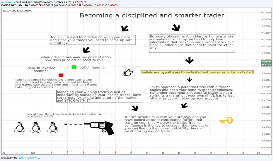
Becoming a disciplined and more thoughtful traderHello there, everyday i look in the chat and i see people making trades based on fomo, chasing price and news and i wanted to bring to life a few steps that i have in place before making a trade. I hope this is helpful! best of luck!