A closer up view of SILJA slighty closer up view of my previously posted SILJ analysis. The yellow could could be off by one degree...in other words the yellow (3) might actually be the teal (3), but either way I see a major move up very very soon...by end of August >$20 imo.
ETF market

Call me crazy....but SILJ looks explosive here...In my opinion we are seeing a series of 1,2's on SILJ which are about to result in a MAJOR move to the upside. IF I am correct then we will see $20+ in very short time...by the end of August!

INDA eyes on $52.64-53.19: Major support could mark the BottomINDA painting a bottom with an inverted Head-n-Shoulders.
The neckline happens to be a fib confluence $52.64-53.19
Good spot to consider longs with stop loss just below zone.
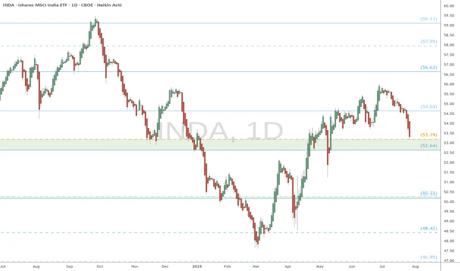
Market Outlook: Bulls are still in control, but be defensive.At theses levels don't let your guard down. I could see us pulling back next week, meanwhile we may continue to stay above the 10-EMA for now.

Nightly $SPY / $SPX Scenarios for July 29, 2025🔮 Nightly AMEX:SPY / SP:SPX Scenarios for July 29, 2025 🔮
🌍 Market‑Moving News 🌍
U.S.–EU Trade Deal Sparks Optimism
The U.S. and EU signed a trade framework allowing a 15% tariff rate on most EU imports, averting harsher penalties. The S&P 500 and Nasdaq both closed at fresh record highs, supported by upbeat tech earnings sentiment—Tesla advanced on a new $16.5B AI chip deal with Samsung—while U.S.–China trade talks resume in Stockholm.
Fed Likely to Hold Rates; Political Pressure Mounts
The Fed is expected to leave its benchmark rate at 4.25%–4.50% at the July 29–30 FOMC meeting. Chair Powell faces growing political pressure from President Trump to cut rates and concerns about central bank independence remain elevated.
Trade Talks Extension to Avoid Tariff Hike Deadline
The August 1 tariff deadline looms. Markets are watching to see if trade deals with China, Canada, and the EU extend the pause or risk new tariffs. Volume in AI/chip stocks and industrials reflects sensitivity to trade developments.
📊 Key Data Releases & Events 📊
📅 Tuesday, July 29
FOMC Meeting Begins — All eyes on Fed rate decision and updated projections.
GDP (Advance Q2 Estimate) — Expected around +1.9% on signs of economic rebound.
⚠️ Disclaimer:
This summary is for educational and informational purposes only—it is not financial advice. Always consult a licensed financial advisor before making investment decisions.
📌 #trading #stockmarket #economy #Fed #trade #tariffs #PCE #jobs #technicalanalysis

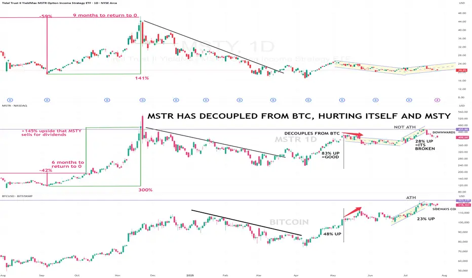
MSTY / MSTRMSTY is mathematically pressured into an exponentially decay relative to MSTR. This chart demonstrates this historical pattern in an obvious way.

PSIL healthy sideways consolidation in very tight rangeHealthy consolidation sideways for three days after breaking through monthly resistance at $17 which we are how holding as support. Volume still meagre, still waiting for this to ramp up significantly to let us know the herd is entering the trade along with us.
Support: 17.03, 16.94, 16.80
Resistance: 17.15, 17.41, 17.60

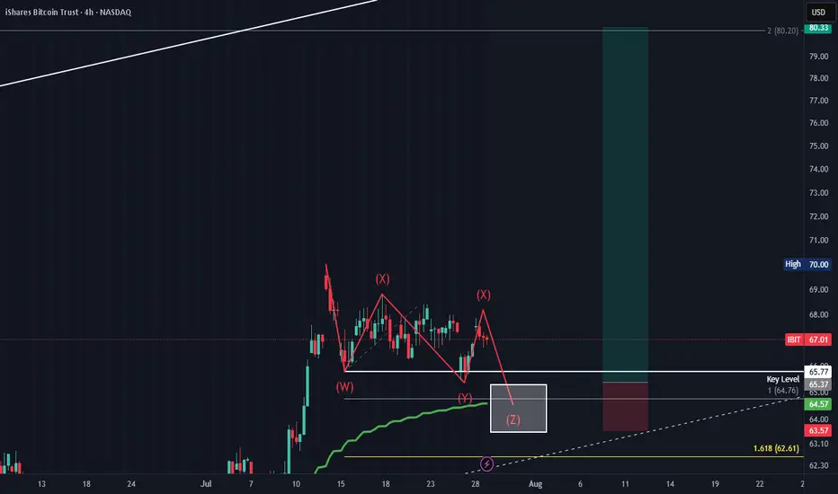
IBIT swing long. WYXYZ corrective pattern.Potential swing long setup. WXYXZ corrective pattern. Taking the lows 1 more time onto the 1 to 1 fib trend. Overall target 80 which should align with BTC hitting 135-150k.
Direxion High Beta Bull S&P 500 3X | HIBL | Long at $30.86Contrarian view, despite tariffs. I don't think this rodeo is over - but I could always be wrong. Even if individual consumption drops (which I think it has for some time now), rising prices will continue to mask it. Many, but not all, companies will profit and until there is a "bigger" catalyst... bullish.
AMEX:HIBL is a personal buy at $30.86 (also noting the possibility of it going into the FWB:20S in the near-term)
Targets:
$40.00
$45.00
$50.00

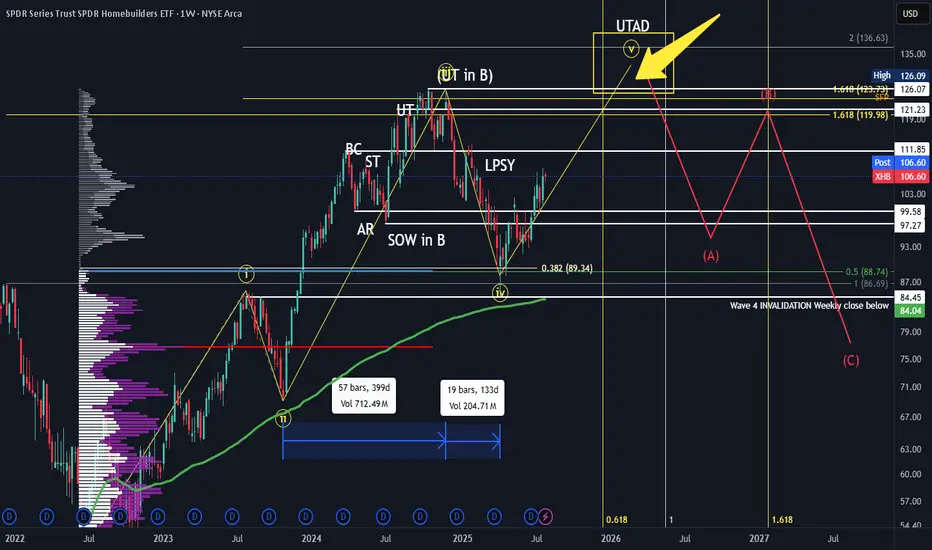
XHB HTF Elliot Wave Count and Wykoff Distribution HTF Elliot Wave Count aligning with HTF Wykoff Distribution Pattern. In confluence with Fibonnacci trend/extension and fibonnaci time. Also further confluence with SPX HTF Wave Count and Distribution
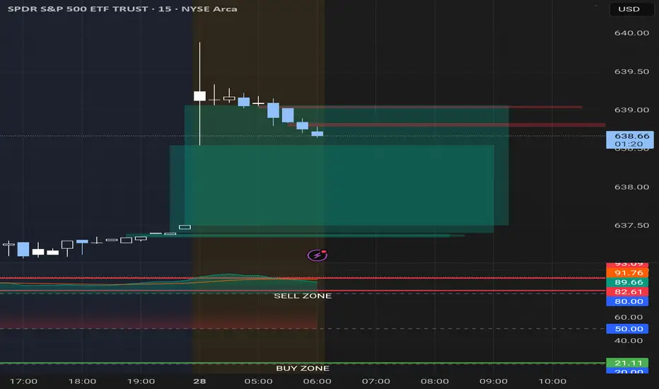
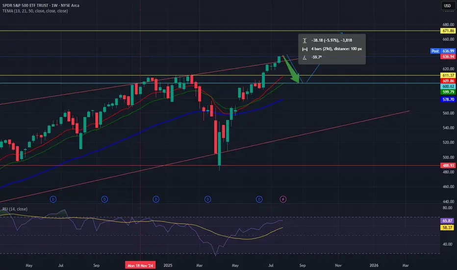
SPY Weekly Chart: Rising Wedge Signals Imminent PullbackSPY Weekly Chart Overview (Current Price: ~637)
🧭 Context:
Indicators: TEMA (13/21/50) & RSI (14)
Price is extended, RSI near overbought (65.87), and forming a rising wedge — a bearish pattern.
🔻 Bearish Setup: Rising wedge signals possible reversal.
Momentum weakening despite higher highs.
Price extended above TEMA — a 600–610 pullback looks likely.
📊 Key Levels:Resistance: 672
Support: 611–600 → 578 → 488
Break below 600 could trigger broad downside.
🟢 Bullish Case:
Breakout above 672 with volume = momentum continuation (AI/FOMO driven).
🎯 Conclusion:
SPY is technically stretched. Risk/reward favors caution.
Watch for pullback to 600–610
XSD watch $243-245: Serious Resistance zone could cause a DipXSD has been grinding up as the chip sector comes back.
About to test a serious resistance zone $243.47-245.96
Look for a Dip-to-Fib or Break-n-Retest for long entries.

SLV Maintains Strong Uptrend AMEX:SLV continues to trade within a strong uptrend, supported by a weakening US Dollar, rising US deficit spending, and growing market uncertainty. Similar to trends observed in precious metals and Bitcoin, the move away from US Treasury Bonds has been a significant bullish catalyst for these assets. Recently, silver prices surged to their highest level in nearly 14 years, and we anticipate further upside potential.
Since reaching a low of $26.57 on April 4th, 2025, AMEX:SLV has been moving within a well-defined upward trending channel. On July 23rd, it posted a new higher high at $35.91, which was met with resistance near the top of the channel at $36.00. This rally was accompanied by a daily RSI reading above 70 and a breakout above the upper Bollinger Band at $35.80—factors that naturally triggered a short-term pullback heading into Friday’s close.
Since then, price action has retraced toward the lower boundary of the channel, now at $34.50, while the daily RSI has returned to long-term trendline support around 57. The upper Bollinger Band has since shifted higher to $36.14. With these technical indicators in place, we anticipate a breakout above the $36.00 level in the near term. As long as AMEX:SLV holds above $34.00, we maintain a bullish outlook with expectations for continued new highs.

Trading as a Probabilistic ProcessTrading as a Probabilistic Process
As mentioned in the previous post , involvement in the market occurs for a wide range of reasons, which creates structural disorder. As a result, trading must be approached with the understanding that outcomes are variable. While a setup may reach a predefined target, it may also result in partial continuation, overextension, no follow-through, or immediate reversal. We trade based on known variables and informed expectations, but the outcome may still fall outside them.
Therefore each individual trade should be viewed as a random outcome. A valid setup could lose; an invalid one could win. It is possible to follow every rule and still take a loss. It is equally possible to break all rules and still see profits. These inconsistencies can cluster into streaks, several wins or losses in a row, without indicating anything about the applied system.
To navigate this, traders should think in terms of sample size. A single trade provides limited insight, relevant information only emerges over a sequence of outcomes. Probabilistic trading means acting on repeatable conditions that show positive expectancy over time, while accepting that the result of any individual trade is unknowable.
Expected Value
Expected value is a formula to measure the long-term performance of a trading system. It represents the average outcome per trade over time, factoring in both wins and losses:
Expected Value = (Win Rate × Average Win) – (Loss Rate × Average Loss)
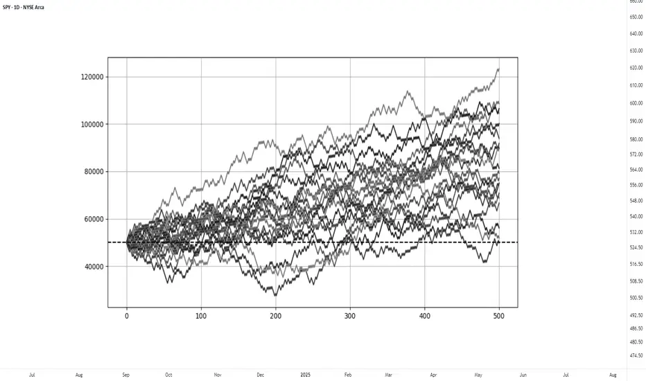
This principle can be demonstrated through simulation. A basic system with a 50% win rate and a 1.1 to 1 reward-to-risk ratio was tested over 500 trades across 20 independent runs. Each run began with a $50,000 account and applied a fixed risk of $1000 per trade. The setup, rules, and parameters remained identical throughout; the only difference was the random sequence in which wins and losses occurred.
While most runs clustered around a profitable outcome consistent with the positive expected value, several outliers demonstrated the impact of sequencing. When 250 trades had been done, one account was up more than 60% while another was down nearly 40%. In one run, the account more than doubled by the end of the 500 trades. In another, it failed to generate any meaningful profit across the entire sequence. These differences occurred not because of flaws in the system, but because of randomness in the order of outcomes.
These are known as Monte Carlo simulations, a method used to estimate possible outcomes of a system by repeatedly running it through randomized sequences. The technique is applied in many fields to model uncertainty and variation. In trading, it can be used to observe how a strategy performs across different sequences of wins and losses, helping to understand the range of outcomes that may result from probability.
Trading System Variations
Two different strategies can produce the same expected value, even if they operate on different terms. This is not a theoretical point, but a practical one that influences what kind of outcomes can be expected.
For example, System A operates with a high win rate and a lower reward-to-risk ratio. It wins 70% of the time with a 0.5 R, while System B takes the opposite approach and wins 30% of the time with a 2.5 R. If the applied risk is $1,000, the following results appear:
System A = (0.70 × 500) − (0.30 × 1,000) = 350 − 300 = $50
System B = (0.30 × 2,500) − (0.70 × 1,000) = 750 − 700 = $50
Both systems average a profit of $50 per trade, yet they are very different to trade and experience. Both are valid approaches if applied consistently. What matters is not the math alone, but whether the method can be executed consistently across the full range of outcomes.
Let’s look a bit closer into the simulations and practical implications.
The simulation above shows the higher winrate, lower reward system with an initial $100,000 balance, which made 50 independent runs of 1000 trades each. It produced an average final balance of $134,225. In terms of variance, the lowest final balance reached $99,500 while the best performer $164,000. Drawdowns remained modest, with an average of 7.67%, and only 5% of the runs ended below the initial $100,000 balance. This approach delivers more frequent rewards and a smoother equity curve, but requires strict control in terms of loss size.
The simulation above shows the lower winrate, higher reward system with an initial $100,000 balance, which made 50 independent runs of 1000 trades each. It produced an average final balance of $132,175. The variance was wider, where some run ended near $86,500 and another moved past $175,000. The drawdowns were deeper and more volatile, with an average of 21%, with the worst at 45%. This approach encounters more frequent losses but has infrequent winners that provide the performance required. This approach requires patience and mental resilience to handle frequent losses.
Practical Implications and Risk
While these simulations are static and simplified compared to real-world trading, the principle remains applicable. These results reinforce the idea that trading outcomes must be viewed probabilistically. A reasonable system can produce a wide range of results in the short term. Without sufficient sample size and risk control, even a valid approach may fail to perform. The purpose is not to predict the outcome of one trade, but to manage risk in a way that allows the account to endure variance and let statistical edge develop over time.
This randomness cannot be eliminated, but the impact can be controlled from position sizing. In case the size is too large, even a profitable system can be wiped out during an unfavorable sequence. This consideration is critical to survive long enough for the edge to express itself.
This is also the reason to remain detached from individual trades. When a trade is invalidated or risk has been exceeded, it should be treated as complete. Each outcome is part of a larger sample. Performance can only be evaluated through cumulative data, not individual trades.
MSTR decouples from BTC, hurting MSTYI use this chart to track BTC, and MSTR so I can safely hold MSTY shares at a price that "should" be safe as long as BTC follows Global Liquidity with a 70-90 day offset (which it IS doing) and MSTR follows BTC price action with a 2x or so, multiplier, (which it WAS, until it decoupled recently). This makes holding MSTY for any share price at $23 or higher, dicey, when MSTR should be in the $500-600 range at the recent BTC ATH and MSTY share price should be in the $30 range, at least. Add to this: BTC is not enjoying the monster 400% runups it had 2021 and previous.
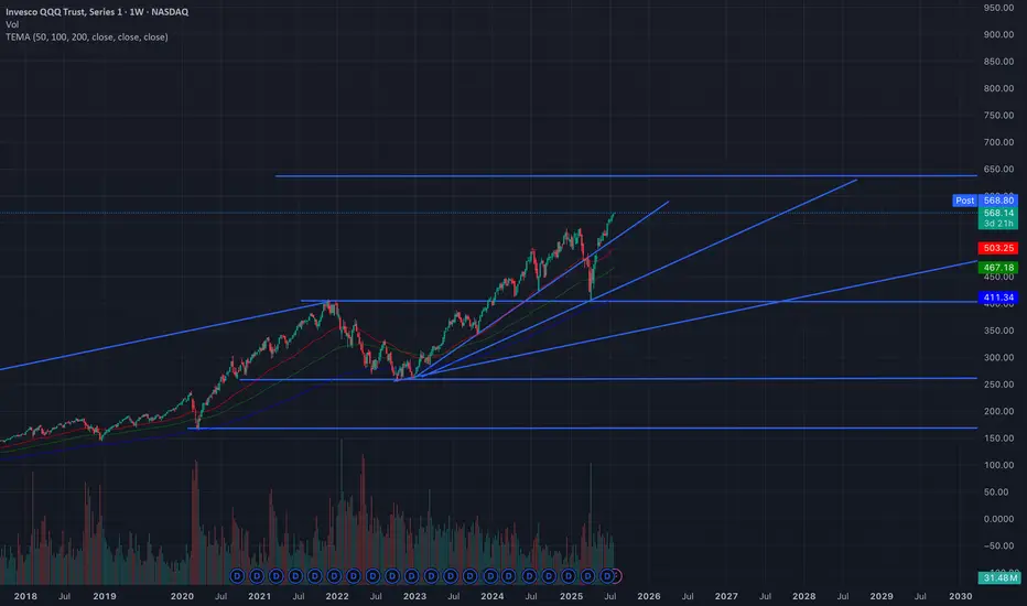
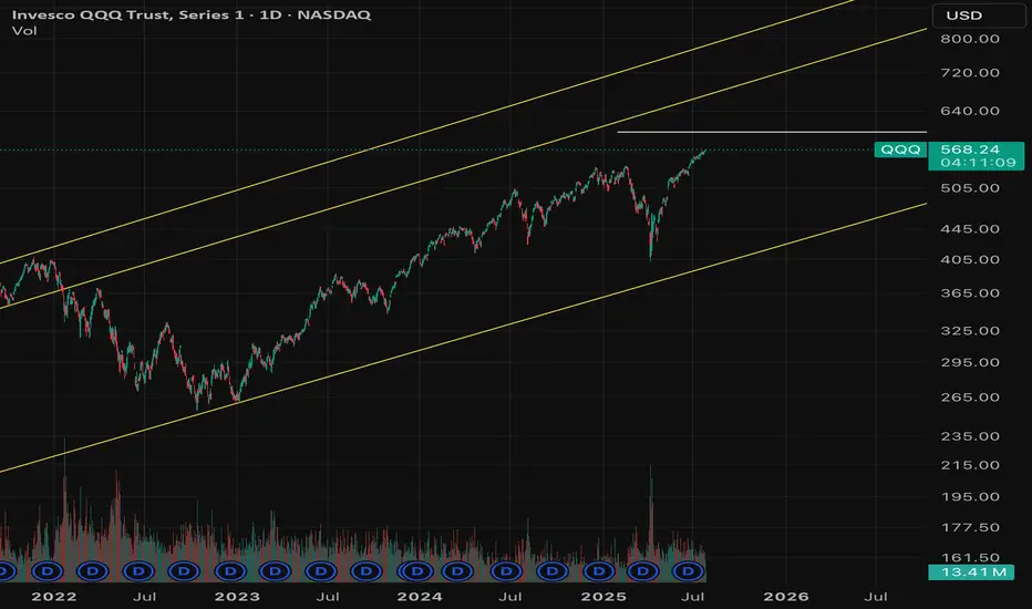
$QQQ August correction incoming?- August correction incoming? 🚨
- Greed is all time highs; People are complacent
- I believe a correction of 5-10% is healthy for the market to flush out excess and remove junk investments from the market.
- This involves people who are over-leveraged gets trapped.
- Personally, taking profits from risky bets, some profits from quality names and raising cash.
- Rotating money to defensive names.
- Not exiting the markets completely.
TQQQ WEEKLY TRADE IDEA (07/28/2025)
**🚀 TQQQ WEEKLY TRADE IDEA (07/28/2025) 🚀**
**Triple-Leveraged Momentum Play — But Watch the Volume Trap!**
---
📈 **Momentum Snapshot:**
* **Daily RSI:** 75.0 ⬆️
* **Weekly RSI:** 70.1 ⬆️
🔥 Bullish across **all timeframes** = strong trend confirmation
📊 **Options Flow:**
* **Call Volume:** 24,492
* **Put Volume:** 18,970
* **C/P Ratio:** **1.29** → Institutional bias = **Bullish**
📉 **Volume Concern:**
* Weekly volume = **0.8x** previous week
⚠️ Weak participation could limit breakout strength
🌪️ **Volatility Environment:**
* **VIX < 20** → ✅ Great for directional plays
---
🔍 **Model Consensus Recap:**
✅ All reports agree on bullish momentum
✅ Favorable volatility = cleaner setups
⚠️ Volume is the only red flag
📌 Final Take: **Bullish, but be tactical**
---
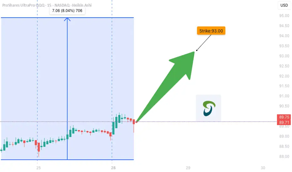
💥 **RECOMMENDED TRADE SETUP (Confidence: 75%)**
🎯 **Play:** Buy CALL Option
* **Strike:** \$93
* **Expiry:** Aug 1, 2025
* **Entry Price:** \~\$0.79
* **Profit Target:** \$1.58 (🟢 2x Gain)
* **Stop Loss:** \$0.39 (🔻 50% Risk)
📆 Entry Timing: Market Open
📏 Position Size: 2–4% of account
---
⚠️ **Key Risks to Watch:**
* 🔍 **Volume Trap**: Weak volume = fragile follow-through
* ⚡ **Gamma Risk** into expiry → price may swing quickly
* 📉 Avoid chasing — stick to setup, use stop-loss
---
📌 **JSON FORMAT TRADE DETAILS (Automation-Ready):**
```json
{
"instrument": "TQQQ",
"direction": "call",
"strike": 93.0,
"expiry": "2025-08-01",
"confidence": 0.75,
"profit_target": 1.58,
"stop_loss": 0.39,
"size": 1,
"entry_price": 0.79,
"entry_timing": "open",
"signal_publish_time": "2025-07-31 09:29:00 UTC-04:00"
}
```
---
**TL;DR:**
✅ RSI momentum = 🔥
📈 Call flow = ✅
⚠️ Volume = 🟡 Caution
🎯 \ NASDAQ:TQQQ breakout play for the bold
💬 Are you riding the 3x bull, or waiting for confirmation?
\#TQQQ #OptionsTrading #MomentumSetup #UnusualOptionsFlow #TradingView #TechStocks #QQQ #LeveragedETF
SPY 15-Min — Weak-High Sweep in Play• Discount BOS at 603.95 → impulsive leg to 606.7 (0.886)
• Weak high tagged at 607.16 – expecting continuation to 1.382 ≈ 608.61 then 1.854 ≈ 610.92
• Invalidation if price closes below 605.45 session VWAP band
• Targets: 608.61 → 610.92
• Risk: stop 604.9 (below 0.5 Fib)
VolanX bias remains risk-on while micro structure stair-steps above the 9-EMA channel.
Educational only – not financial advice
#SPY #SMP500 #OrderFlow #Fib #VolanX #WaverVanir

SPY: Aiming 626 today Slowly./ Let's observe what this market will give us. If there is a setup, we take the trade.

Semiconductors & SOXL: A Bull ThesisWhy Semiconductors?
Virtually every single electronic device contains some form of a semiconductor unit within its components. The entire Bull theory on semiconductors as an industry could be reduced to this one sentence. The following, however, will introduce concepts contingent to the understanding of what is shaping the market for semiconductors. The weight of intra-industry, political, macroeconomic, and physical factors discerning an inconceivable upside potential for certain investments carrying maximum exposure to the sector, such as AMEX:SOXL . The last section contains my technical approach to trading SOXL.
We begin with the fundamental, and by fundamental, I refer to the simplest reasons for what is happening in the market up until now; [ Early morning Monday, 7/28 ].
Macroeconomic Context
Like essentially the rest of the market, SOXL hit its 1 year low of 7.23 USD on Monday, 4/7, following the announcement (and soon postponement) of global tariffs at levels not observed since the early 30's. This of course sparked a panic spiral in the entire market, leading to outflows from the S&P 500 of approximately 70 billion USD during the month of April. During this time we also saw a new, but familiar narrative emerge. Asset Managers, Such as J.P. Morgan set historically low price targets on the S&P 500, going as low as 5,200 USD. They reinforced their PTs with publications warning investors across the world that the risk of recession in the United States was raised to 80%, and this message was relayed across all media in parabolic fashion. While it does not seem too outward to assume an increased risk of recession due to tariffs by looking back on what we learned of the consequences from the Smoot-Hawley Tariff Act of 1930. There exists a widely overlooked, fundamental , reason as to why I can claim that the REAL risk of recession at the time that J.P. Morgan assigned an 80% risk of recession, was in actuality, 0% (I assume J.P. Morgan knew this but pushed the narrative anyways in order to acquire massive equity at a discount). If anyone has taken introductory macroeconomics in their lifetime, they may be familiar with the function for calculating GDP via the expenditure approach: GDP = C + I + G - NX. Now, why am I referencing high school/college economics basics, the answer to that lies in how we determine our rate of economic growth in the context of tariffs. The part of this formula that we must focus on is NX or Net Exports, the negative factor to GDP. Tariffs, if implemented would effectively decrease import volume, resulting in a smaller Net Exports, and ultimately a higher GDP calculation. Now, what makes this scenario unique, the tariffs having been postponed shortly after their inception, allowed US retailers to engage in front running, or the accelerated purchasing of foreign goods in advance of tariffs. During the month of April, we saw a 5.4% increase in import volume in US west coast ports. This increase in imports effectively caused the inverse impact on GDP growth that import tariffs themselves would have caused: front-running lead to import uptick, leading to a greater Net Exports, which results in lower (negative) GDP growth. Essentially, tariffs in the short-term increases GDP growth (in the long term deadweight loss, and cost structure distortion comes in to play, but that doesn't matter yet), however , tariffs that are announced but not immediately implemented will result in a lower GDP growth, coupled with uncertainty surrounding the whole situation that translated into a cut in CapEx as companies scrambled to determine if tariffs would f*ck them over or not. This argument is further supported by the trends observed in the foreign exchange market. You may have heard in the news that we are experiencing a period of "Dollar Weakness", and while, yes, you can clearly see that the USD has fared rather poorly against other currencies in most major dollar pairs over the past few months. The agent behind this isn't just that the dollar happens to be weak, it is a combination of factors that generate noise and volatility in the forex market. The two main factors highlighted by the media are 1. The obvious political policy instability, pushing bond yields higher, plus a significant debt ceiling raise as per the BBB and 2. the expectations of interest rate cuts over the next year. The other, less recognized major factor to dollar weakness is exactly what we described above: Increased imports means more dollars flowing out of the economy. When these dollars land abroad, they are converted into the native currency, driving down the demand for the dollar. Notice how none of the reasons described above, actually have anything to do with what truly drives foreign exchange markets. Over time, the strength/weakness of a currency is directly correlated to the strength/weakness of the underlying economy. To say that we can expect dollar weakness due to the aforementioned reasons outright ignores the economic growth potential that exists in our economy at this current time, subsiding the out-of-proportion tariff fears as a proponent to an economic crisis. In an all-encompassing view, what I would describe to be occurring on the macro level is a sort of "slingshot" effect: Trade imbalances and private sector response to policy unclarity results in a pullback in economic growth, one that we are now experiencing as a short-term effect. From a medium-long term perspective, assuming that tariffs aren't persistent in the long term, we would see full fledge economic boom, driven by non other than the growth of our technology sector, which at it's core, lies the almighty semiconductor.
Growth of AI as a driver of Semiconductor demand: Stable trajectory or Bubble Territory?
Having laid the economic framework for picking the general direction our market is heading in, we can now begin to talk about the internal combustion occurring within the world of technology, and the two letter term associated with just about every cool thing in the business world, that is of course AI. Now just to clarify, AI is not new, its been around for at least 20 years and has a well established role in the world prior to the existence of ChatGPT. What changed so drastically in recent years is the breakthrough into a new form of artificial intelligence, known as "Artificial General Intelligence" or AGI. Long story short: AGI's primary difference in the business context is the colossal amount of electrical infrastructure and computing power that is demanded by the development of these mega language models. As a result of the high barrier for entry to this new industry, only 5 AGI companies have arisen to the global stage: OpenAI, Google DeepMind, Anthropic, Microsoft, and DeepSeek. Increasing competition in this space through more players entering the market is unlikely at this time as the cost to create a standalone AGI model is so astronomical. This is a particularly good thing because it tells us that AGI as an industry can result in natural monopolies. The ultra-intensive RnD costs and Data Center infrastructure demands make it more sensical to have a greater number of resources dedicated to producing 1 AGI model, instead of dividing resources to develop multiple less optimized models (similar to how a water company holds a natural monopoly as competition in that industry would result in no foreseeable benefit to it's customers). A further effect from this dynamic lies in how businesses in this industry scale to expand, and its pretty straightforward: the more megawatt computing power a model can access, the more parameters a model can account for, and the more vast the dataset that model can train on, with enhancing speed and efficiency (GPT 4o takes into account >500B parameters in a given query). We see the concept of natural monopoly playing out as the concentration of market capitalization is becoming more extreme where firms like Google, Microsoft, and NVIDIA are absorbing larger share of the market, while trading at ever increasing Price/Earnings multiples. To many, this reflects a trend we saw during the dot com bubble, however what makes the AGI industry different is the nature of the good or service provided. During the dot com boom, companies saw speculative value based on only the fact that their business existed on the .com domain. We know that each of these businesses are unique, providing a good or service across whatever industry they were part of, the only thing having in common was that dot com. The major oversight that took place during the turn of the dot com era was that the success of these businesses wasn't in truth due to them ending in .com, but whether the idea, and execution behind the underlying business is strong or not. Like how Amazon and Facebook saw unparalleled success not just because they were .coms, but because they were pioneering business models that would attract global demand to the services they were providing. The business of AGI has a sort of homogenous property. All AGI companies produce a service that is extremely similar in nature, the only ways they can compete with one another is through Capital Expenditure towards harnessing more computing power. This is the main reason capital is concentrating in a handful of companies trading at high multiples. To me, this is not an indication of a tech bubble but rather a product of how the AGI industry is poised to grow within our economy.
AGI as a Factor of Production
To get even more philosophical, we can think about how AGI itself enhances economic growth. We already see AGI tools applied in various ways, but the most widespread application pertains to the enhancement of human capital. While it is possible to make AGI models complete ongoing tasks completely on their own with zero human input, its far more common to see AGI tools be used, well, as tools. What I mean is that firms are not looking to replace human workers with AI ones (certain exceptions may include the manufacturing industry), instead they want to integrate AGI tools into their workforce as a means of optimizing regular processes, allowing them to access and process information with tremendous efficiency. The most observable economic outcome of this is firms being able to cut costs in human capital requirements, allowing them to achieve the same level of workflow with a smaller number of employees, or outsourcing solutions to business processes by way of automation utilizing AGI. The possibilities are endless and the economic impact of AGI appears to write itself new economic theory to explain how business growth is accelerating in unprecedented ways.
Semiconductor Physical Limitations: Blessing or Burden?
In 1965, Gordon Moore articulated his observation which would come to be known as Moore's Law. He observed that the number of transistors in an integrated circuit doubles approximately every 2 years. Based not so much on law of physics, Moore's law describes an empirical relationship between time and the number of transistors per chip, suggesting that the rate of production advancements would allow for such doubling to occur on a biannual basis. And to Gordon's own surprise, he was right. Transistor count for a given chip roughly doubled every 2 years for the following 50 years. However, Gordon also predicted that Moore's Law would come to an end in 2025, where transistor sizes would reach the physical limit of 2 nanometers (10-15 silicon atoms in width). While it may appear as a bottleneck to the semiconductor and AI industry, not being able to fit anymore transistors on one chip, but in reality, this limitation pressures companies to pursue innovations such as semiconductor packaging, which is NVIDIA's bread and butter. This technique allows for the stacking and integrating of many different chips to perform together as one. This technology has already proven wildly successful and is the backbone to virtually all of NVIDIA's GPU products. Google has invented their own method to getting around the physical limitation of silicon chips, producing AI-specialized integrated circuits known as Tensor Processing Units (TPUs). Catering these innovative solutions to expanding the frontier of AGI is almost a given.
How to play this market: A Technical Approach
If you have made it this far, I commend you. The following describes my approach to analyzing price activity in SOXL:
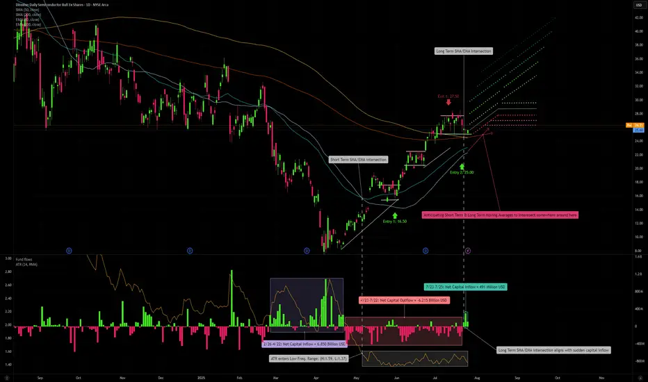
My First entry into SOXL took place on 5/30 with a unit cost of 16.50 USD. Two things can be noted prior to this entry. 1: Fund flows during late February, into March, and through April were extremely high, net inflow of 6.85 Billion USD, however price movement did not reflect the huge inflow until late April/early May where we began to see upward price direction. The beginning of June marked the start of the market bull rally which consolidated into our current price range of 25-28 USD, following contingent earnings releases of NASDAQ:ASML , NYSE:TSM , NASDAQ:NXPI and NASDAQ:INTC . The most recent pullback was a combination of a slightly concerning outlook from ASML, stating that tariffs on the EU would negatively affect projected sales growth for the 2026 fiscal year. As for TSM, there is not one concerning thing that could be said regarding the state of its business growth other than the New Taiwan Dollar gaining considerable strength over the USD amid trade relations between the US and Taiwan, affecting TSM's gross margin by an estimated 6%. NXPI released a sub par earnings and revenue growth outlook, but in my opinion this is not to be too heavily objectified as NXPI produces chips primarily for the Automotive sector, thus making it's sales heavily contingent on supply chain issues being faced by automotive manufacturers in leu of tariffs. NXPI carries a 3.5% market share in semiconductors whereas TSM carries a 68% market share. Lastly, INTC, earnings release I am almost embarrassed to talk about. If it were up to me I'd say they sell their plants in Ohio to TSM and look into opening a fruit stand instead. The most important earnings releases have yet to come though. NASDAQ:MSFT is just around the corner on 7/30, and NASDAQ:NVDA announces on 8/27. These two earnings reports will carry major weight in hinting the overall direction, momentum the market sees in AI demand growth, and the technology sector as a whole. Speculating, I have high expectations that both MSFT and NVDA will top all estimates, pushing the bar higher for 2025 into 2026.
If we look at our short-term 50-day SMA/EMA, you will notice a crossover occur on 5/6, a minor indication of a short term positive trend. Alone this is insignificant, but if we look at our 14-day Average True Range, we can see that this crossover aligns with a fall in ATR that would persist between the values of 1.37 and 1.59. This low ATR value signals that trailing volatility is actually quite low for semiconductors, considering the currently mixed market sentiment. Further along we see that price has crossed above both our long-term, 200-day SMA/EMA and a crossover occurred between the two on 7/23, serving as a small indication of a positive long term trend. Once again, not super significant on its own, but you will notice that the convergence aligns perfectly with a sharp increase in fund inflows, netting 491 Million USD in a matter of 3 trading days. If we see a continuation of net inflows over the several days, we can expect a near future extension of our bull rally, a semi-cyclical wave of inflows that concentrate during consolidation periods (which we have seen take place in the current price range between 25-28 USD following my first exit at 27.50 USD). If we extrapolate both our short-term and long-term SMA/EMA, we can anticipate a crossover to occur in the coming days to weeks. If this occurred, that would further reinforce our expectation for a positive long term trend. I have already locked in my entry 2 with a limit order executed at 25 USD. If all of the above conditions are met, I would confidently predict that we may see SOXL trade at around 42 USD in the coming months.
One more thing I would like to note, if we zoom out to our 5 year historical price progression, we can identify the previous high of 70.08 USD occurring on 7/11/2024. We know that the bull rally which took place in July of last year can be attributed to the first realization of AI as a driver for semiconductor demand, combined with renewed interest in GPU technology for applications in crypto. If we compare AI-related Capital Expenditure in fiscal year 2024 to AI-related Capital Expenditure of the first half of 2025 fiscal year: 246 Billion USD made up AI-related CapEx for all of 2024, vs first 6 months of 2025, adding up to 320 Billion USD. That is a 30% increase in capex, and we still have another 5-6 months to go. Just some food for thought.
Do you believe all of the above has been priced into SOXL, leave your thoughts in the comments!
Disclaimer
You must obviously keep in mind, SOXL is a 3x leveraged ETF, you can expect volatility with such type of investment. However, in capturing a bullish market, a 3x leveraged investment may produce greater than 3x the returns as the underlying (non leveraged) assets, due to the effect of compounding growth of returns over time. However, the same is true for sideways, or bearish markets, losses may be amplified to greater than 3x. If this is an uncertainty you do not wish to be exposed to, I would opt for the non-leveraged Semiconductor ETF ( NASDAQ:SOXX ), or divide your allocation across the top 5-10 equity holdings of SOXL. Please remember to employ your OWN due diligence before making any investment decision, as none of what I am saying shall serve as financial advise to you, the reader.
Are you ready for this scenario?? BUY THE NEXT BOTTOM!!!Spx is gonna drop hard, are you ready to buy the next bottom?
I expect SPX to reach 4,440 atleast... NASDAQ, BITCOIN are gonna drop hard too...
BUY EVERYTHING IN 2026/2027 AND ENJOY THE NEXT CYCLE.

Play I am looking at.Golden cross starting to line up on VVIX on the 10 and 15min. If VIX spikes we could fill the Gap on SPY making it a perfect set up as it will also lign it up for a rebound off the 200MA. Depending on what the level 2 says at that time ill be loading 640 calls and 643Calls. I'll take a speculative guess that it SPY will open with short formed W pattern off that MA.