Combo 2/20 EMA & Bandpass Filter by TamarokDescription:
This strategy combines a 2/20 exponential moving average (EMA) crossover with a custom bandpass filter to generate buy and sell signals.
Use the Fast EMA and Slow EMA inputs to adjust trend sensitivity, and the Bandpass Filter Length, Delta, and Zones to fine-tune momentum turns.
Signals occur when both EMA and BPF agree in direction, with optional reversal and time filters.
How to use:
1. Add the script to your chart in TradingView.
2. Adjust the EMA and BP Filter parameters to match your asset’s volatility.
3. Enable ‘Reverse Signals’ to trade counter-trend, or use the time filter to limit sessions.
4. Set alerts on Long Alert and Short Alert for automated notifications.
Inspiration:
Based on HPotter’s original combo strategy (Stocks & Commodities Mar 2010).
Updated to Pine Script v6 with streamlined code and alerts.
WARNING:
For purpose educate only
Filter

Kent Directional Filter🧭 Kent Directional Filter
Author: GabrielAmadeusLau
Type: Filter
📖 What It Is
The Kent Directional Filter is a directionality-sensitive smoothing tool inspired by the Kent distribution, a probability model used to describe directional and elliptical shapes on a sphere. In this context, it's repurposed for analyzing the angular trajectory of price movements and smoothing them for actionable insights.
It’s ideal for:
Detecting directional bias with probabilistic weighting
Enhancing momentum or trend-following systems
Filtering non-linear price action
🔬 How It Works
Price Angle Estimation:
Computes a rough angular shift in price using atan(src - src ) to estimate direction.
Kent Distribution Weighting:
κ (kappa) controls concentration strength (how sharply it prefers a direction).
β (beta) controls ellipticity (bias toward curved vs. linear moves).
These parameters influence how strongly the indicator favors movements at ~45° angles, simulating a directional “lens.”
Smoothing:
A Simple Moving Average (SMA) is applied over the raw directional probabilities to reduce noise and highlight the underlying trend signal.
⚙️ Inputs
Source: Price series used for angle calculation (default: close)
Smoothing Length: Window size for the moving average
Pi Divisor: Pi / 4 would be 45 degrees, you can change the 4 to 3, 2, etc.
Kappa (κ): Controls how focused the directionality is (higher = sharper filter)
Beta (β): Adds curvature sensitivity; higher values accentuate asymmetrical moves
🧠 Tips for Best Results
Use κ = 1–2 for moderate directional filtering, and β = 0.3–0.7 for smooth elliptical bias.
Combine with volume-based indicators to confirm breakout strength.
Works best in higher timeframes (1h–1D) to capture macro directional structure.
I might revisit this.

TASC 2025.07 Laguerre Filters█ OVERVIEW
This script implements the Laguerre filter and oscillator described by John F. Ehlers in the article "A Tool For Trend Trading, Laguerre Filters" from the July 2025 edition of TASC's Traders' Tips . The new Laguerre filter utilizes the UltimateSmoother filter in place of an exponential moving average (EMA) in its calculation, offering improved responsiveness and reduced lag.
█ CONCEPTS
As Ehlers explains in his article, the Laguerre filter is a form of transversal filter . A transversal filter calculates an output signal using a tapped delay line . It creates multiple delayed versions of an input signal, applies weight to each delay, and then calculates their sum to generate the filtered result.
The Laguerre filter's structure relies on Laguerre polynomials — solutions to a differential equation solved by Edmond Laguerre in the 1800s. When Ehlers analyzed the formula for these polynomials on discrete systems (e.g., financial time series), he found that the first term's expression corresponds to an EMA response, and all subsequent terms correspond to an all-pass response. In contrast to other filter types, an all-pass filter produces phase shift (i.e., delay) in an input signal's components without affecting its amplitude.
Ehlers observed that these characteristics of Laguerre polynomials make them suitable for use in a transversal filter structure, and thus the Laguerre filter was born. However, he notes that EMAs are not great filters in general. As such, to improve on the Laguerre filter's design, Ehlers modified it by replacing the EMA term with his UltimateSmoother filter. The resulting Laguerre filter has significantly reduced lag, achieving a tighter response to market fluctuations while maintaining smoothness. Ehlers suggests that traders can analyze crossings between the UltimateSmoother and this Laguerre filter, or those between two Laguerre filters of different order, for helpful buy and sell signals.
In addition to the Laguerre filter, Ehlers derived a smooth, low-lag oscillator based on the difference between the first and second terms in the modified filter structure, scaled by the root mean square (RMS). The resulting oscillator provides an alternative filtered representation of market data, which can help traders identify swing and mean-reversion signals.
█ USAGE
This indicator calculates both the Laguerre filter and the Laguerre oscillator described in Ehlers' article. It displays the Laguerre filter on the main chart pane and the oscillator in a separate pane.
Users can control the behavior of the filter and oscillator with the inputs in the "Settings/Inputs" tab:
The "Period" input defines the critical period of the UltimateSmoother used in the Laguerre filter and oscillator calculations. Its default value is 30.
The "Gamma" input determines the weighting behavior of the Laguerre filter and oscillator. It accepts a positive value between 0 and 1. Use a lower value for quicker responsiveness to market changes, and a higher value for trends. The default value is 0.5.
The "RMS length" input determines the length of the RMS calculation for oscillator normalization. The default value is 100 bars.

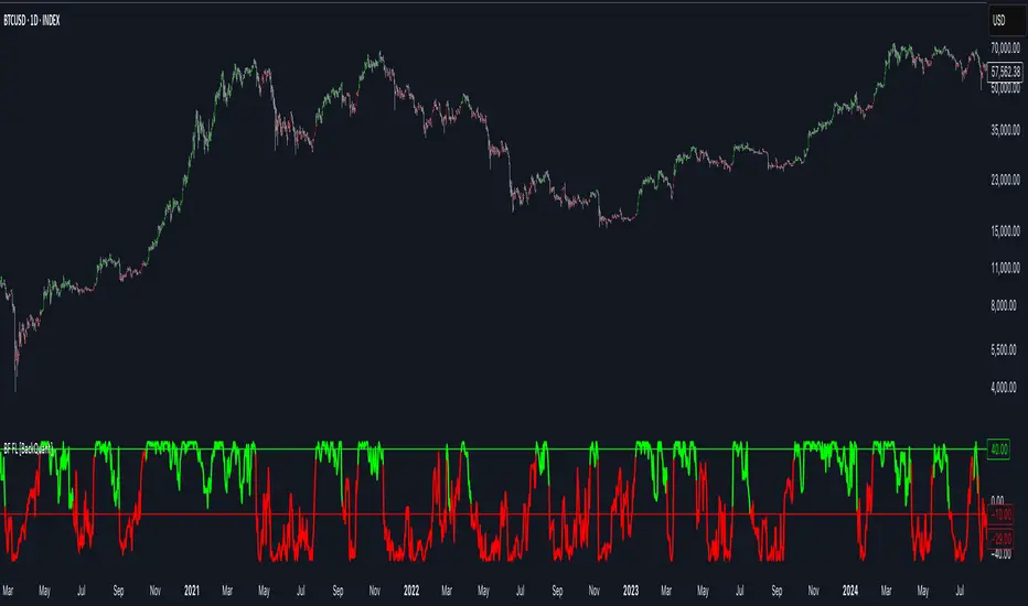
Bilateral Filter For Loop [BackQuant]Bilateral Filter For Loop
The Bilateral Filter For Loop is an advanced technical indicator designed to filter out market noise and smooth out price data, thus improving the identification of underlying market trends. It employs a bilateral filter, which is a sophisticated non-linear filter commonly used in image processing and price time series analysis. By considering both spatial and range differences between price points, this filter is highly effective at preserving significant trends while reducing random fluctuations, ultimately making it suitable for dynamic trend-following strategies.
Please take the time to read the following:
Key Features
1. Bilateral Filter Calculation:
The bilateral filter is the core of this indicator and works by applying a weight to each data point based on two factors: spatial distance and price range difference. This dual weighting process allows the filter to preserve important price movements while reducing the impact of less relevant fluctuations. The filter uses two primary parameters:
Spatial Sigma (σ_d): This parameter adjusts the weight applied based on the distance of each price point from the current price. A larger spatial sigma means more smoothing, as further away values will contribute more heavily to the result.
Range Sigma (σ_r): This parameter controls how much weight is applied based on the difference in price values. Larger price differences result in smaller weights, while similar price values result in larger weights, thereby preserving the trend while filtering out noise.
The output of this filter is a smoothed version of the original price series, which eliminates short-term fluctuations, helping traders focus on longer-term trends. The bilateral filter is applied over a rolling window, adjusting the level of smoothing dynamically based on both the distance between values and their relative price movements.
2. For Loop Calculation for Trend Scoring:
A for-loop is used to calculate the trend score based on the filtered price data. The loop compares the current value to previous values within the specified window, scoring the trend as follows:
+1 for upward movement (when the filtered value is greater than the previous value).
-1 for downward movement (when the filtered value is less than the previous value).
The cumulative result of this loop gives a continuous trend score, which serves as a directional indicator for the market's momentum. By summing the scores over the window period, the loop provides an aggregate value that reflects the overall trend strength. This score helps determine whether the market is experiencing a strong uptrend, downtrend, or sideways movement.
3. Long and Short Conditions:
Once the trend score has been calculated, it is compared against predefined threshold levels:
A long signal is generated when the trend score exceeds the upper threshold, indicating that the market is in a strong uptrend.
A short signal is generated when the trend score crosses below the lower threshold, signaling a potential downtrend or trend reversal.
These conditions provide clear signals for potential entry points, and the color-coding helps traders quickly identify market direction:
Long signals are displayed in green.
Short signals are displayed in red.
These signals are designed to provide high-confidence entries for trend-following strategies, helping traders capture profitable movements in the market.
4. Trend Background and Bar Coloring:
The script offers customizable visual settings to enhance the clarity of the trend signals. Traders can choose to:
Color the bars based on the trend direction: Bars are colored green for long signals and red for short signals.
Change the background color to provide additional context: The background will be shaded green for a bullish trend and red for a bearish trend. This visual feedback helps traders to stay aligned with the prevailing market sentiment.
These features offer a quick visual reference for understanding the market's direction, making it easier for traders to identify when to enter or exit positions.
5. Threshold Lines for Visual Feedback:
Threshold lines are plotted on the chart to represent the predefined long and short levels. These lines act as clear markers for when the market reaches a critical threshold, triggering a potential buy (long) or sell (short) signal. By showing these threshold lines on the chart, traders can quickly gauge the strength of the market and assess whether the trend is strong enough to warrant action.
These thresholds can be adjusted based on the trader's preferences, allowing them to fine-tune the indicator for different market conditions or asset behaviors.
6. Customizable Parameters for Flexibility:
The indicator offers several parameters that can be adjusted to suit individual trading preferences:
Window Period (Bilateral Filter): The window size determines how many past price values are used to calculate the bilateral filter. A larger window increases smoothing, while a smaller window results in more responsive, but noisier, data.
Spatial Sigma (σ_d) and Range Sigma (σ_r): These values control how sensitive the filter is to price changes and the distance between data points. Fine-tuning these parameters allows traders to adjust the degree of noise reduction applied to the price series.
Threshold Levels: The upper and lower thresholds determine when the trend score crosses into long or short territory. These levels can be customized to better match the trader's risk tolerance or asset characteristics.
Visual Settings: Traders can customize the appearance of the chart, including the line width of trend signals, bar colors, and background shading, to make the indicator more readable and aligned with their charting style.
7. Alerts for Trend Reversals:
The indicator includes alert conditions for real-time notifications when the market crosses the defined thresholds. Traders can set alerts to be notified when:
The trend score crosses the long threshold, signaling an uptrend.
The trend score crosses the short threshold, signaling a downtrend.
These alerts provide timely information, allowing traders to take immediate action when the market shows a significant change in direction.
Final Thoughts
The Bilateral Filter For Loop indicator is a robust tool for trend-following traders who wish to reduce market noise and focus on the underlying trend. By applying the bilateral filter and calculating trend scores, this indicator helps traders identify strong uptrends and downtrends, providing reliable entry signals with minimal market noise. The customizable parameters, visual feedback, and alerting system make it a versatile tool for traders seeking to improve their timing and capture profitable market movements.
Thus following all of the key points here are some sample backtests on the 1D Chart
Disclaimer: Backtests are based off past results, and are not indicative of the future.
INDEX:BTCUSD
INDEX:ETHUSD
CRYPTO:SOLUSD
Wavelet Filter with Adaptive Upsampling [BackQuant]Wavelet Filter with Adaptive Upsampling
The Wavelet Filter with Adaptive Upsampling is an advanced filtering and signal reconstruction tool designed to enhance the analysis of financial time series data. It combines wavelet transforms with adaptive upsampling techniques to filter and reconstruct price data, making it ideal for capturing subtle market movements and enhancing trend detection. This system uses high-pass and low-pass filters to decompose the price series into different frequency components, applying adaptive thresholding to eliminate noise and preserve relevant signal information.
Shout out to Loxx for the Least Squares fitting of trigonometric series and Quinn and Fernandes algorithm for finding frequency
www.tradingview.com
Key Features
1. Frequency Decomposition with High-Pass and Low-Pass Filters:
The indicator decomposes the input time series using high-pass and low-pass filters to separate the high-frequency (detail) and low-frequency (trend) components of the data. This decomposition allows for a more accurate analysis of underlying trends, while mitigating the impact of noise.
2. Soft Thresholding for Noise Reduction:
A soft thresholding function is applied to the high-frequency component, allowing for the reduction of noise while retaining significant market signals. This function adjusts the coefficients of the high-frequency data, removing small fluctuations and leaving only the essential price movements.
3. Adaptive Upsampling Process:
The upsampling process in this script can be customized using different methods: sinusoidal upsampling, advanced upsampling, and simple upsampling. Each method serves a unique purpose:
Sinusoidal Upsample uses a sine wave to interpolate between data points, providing a smooth transition.
Advanced Upsample utilizes a Quinn-Fernandes algorithm to estimate frequency and apply more sophisticated interpolation techniques, adapting to the market’s cyclical behavior.
Simple Upsample linearly interpolates between data points, providing a basic upsampling technique for less complex analysis.
4. Reconstruction of Filtered Signal:
The indicator reconstructs the filtered signal by summing the high and low-frequency components after upsampling. This allows for a detailed yet smooth representation of the original time series, which can be used for analyzing underlying trends in the market.
5. Visualization of Reconstructed Data:
The reconstructed series is plotted, showing how the upsampling and filtering process enhances the clarity of the price movements. Additionally, the script provides the option to visualize the log returns of the reconstructed series as a histogram, with positive returns shown in green and negative returns in red.
6. Cumulative Series and Trend Detection:
A cumulative series is plotted to visualize the compounded effect of the filtered and reconstructed data. This feature helps traders track the overall performance of the asset over time, identifying whether the asset is following a sustained upward or downward trend.
7. Adaptive Thresholding and Noise Estimation:
The system estimates the noise level in the high-frequency component and applies an adaptive thresholding process based on the standard deviation of the downsampled data. This ensures that only significant price movements are retained, further refining the trend analysis.
8. Customizable Parameters for Flexibility:
Users can customize the following parameters to adjust the behavior of the indicator:
Frequency and Phase Shift: Control the periodicity of the wavelet transformation and the phase of the upsampling function.
Upsample Factor: Adjust the level of interpolation applied during the upsampling process.
Smoothing Period: Determine the length of time used to smooth the signal, helping to filter out short-term fluctuations.
References
Enhancing Cross-Sectional Currency Strategies with Context-Aware Learning to Rank
arxiv.org
Daubechies Wavelet - Wikipedia
en.wikipedia.org
Quinn Fernandes Fourier Transform of Filtered Price by Loxx
Note on Usage for Mean-Reversion Strategy
This indicator is primarily designed for trend-following strategies. However, by taking the inverse of the signals, it can be adapted for mean-reversion strategies. This involves buying underperforming assets and selling outperforming ones. Caution: This method may not work effectively with highly correlated assets, as the price movements between correlated assets tend to mirror each other, limiting the effectiveness of mean-reversion strategies.
Final Thoughts
The Wavelet Filter with Adaptive Upsampling is a powerful tool for traders seeking to improve their understanding of market trends and noise. By using advanced wavelet decomposition and adaptive upsampling, this system offers a clearer, more refined picture of price movements, enhancing trend-following strategies. It’s particularly useful for detecting subtle shifts in market momentum and reconstructing price data in a way that removes noise, providing more accurate insights into market conditions.

WLSMA: fast approximation🙏🏻 Sup TV & @alexgrover
O(N) algocomplexity, just one loop inside. No, you can't do O(1) @ updates in moving window mode, only expanding window will allow that.
Now I have time series & stats models of my own creation, nowhere else available, just TV and my github for now, ain’t no legacy academic industry I always have fun about, but back in 2k20 when I consciously ain’t known much about quant, I remember seeing post by @alexgrover recreating Moving Regression Endpoint dropped on price chart (called LSMA here) as a linear filter combination of filters (yea yeah DSP terms) as 3WMA - 2SMA. Now it’s my time to do smth alike aye?
...
This script is remake of my 1st degree WLSMA via linear filter combo. It’s much faster, we aint calculate moving regression per se, we just match its freq response. You can see it on the screen (WLSMAfa) almost perfectly matching the original one (WLSMA).
...
While humans like to overfit, I fw generalizations. So your lovely WMA is actually just one case of a more general weight pattern: pow(len - i, e), where pow is the power function and e is the exponent itself. So:
- If e = 0, then we have SMA (every number in 0th power is one)
- If e = 1, we get WMA
- If e = 2, we get quadratic weights.
We can recreate WLSMA freq response then by combining 2 filters with e = 1 and e = 2.
This is still an approximation, even tho enormously precise for the tasks you’ve shared with me. Due to the non-linear nature of the thing it’s all we can do, and as window size grows, even this small discrepancy converges with true WLSMA value, so we’re all good. Pls don’t try to model this 0.00xxxx discrepancy, it’s not natural.
...
DSP approach is unnatural for prices, but you can put this thing on volume delta and be happy, or on other metrics of yours, if for some reason u dont wanna estimate thresholds by fitting a distro.
All good TV
∞
P.S.: strangely, the first script made & dropped in the location in Saint P where my actual quant way has started ~5 years ago xD, very thankful

TASC 2025.06 Cybernetic Oscillator█ OVERVIEW
This script implements the Cybernetic Oscillator introduced by John F. Ehlers in his article "The Cybernetic Oscillator For More Flexibility, Making A Better Oscillator" from the June 2025 edition of the TASC Traders' Tips . It cascades two-pole highpass and lowpass filters, then scales the result by its root mean square (RMS) to create a flexible normalized oscillator that responds to a customizable frequency range for different trading styles.
█ CONCEPTS
Oscillators are indicators widely used by technical traders. These indicators swing above and below a center value, emphasizing cyclic movements within a frequency range. In his article, Ehlers explains that all oscillators share a common characteristic: their calculations involve computing differences . The reliance on differences is what causes these indicators to oscillate about a central point.
The difference between two data points in a series acts as a highpass filter — it allows high frequencies (short wavelengths) to pass through while significantly attenuating low frequencies (long wavelengths). Ehlers demonstrates that a simple difference calculation attenuates lower-frequency cycles at a rate of 6 dB per octave. However, the difference also significantly amplifies cycles near the shortest observable wavelength, making the result appear noisier than the original series. To mitigate the effects of noise in a differenced series, oscillators typically smooth the series with a lowpass filter, such as a moving average.
Ehlers highlights an underlying issue with smoothing differenced data to create oscillators. He postulates that market data statistically follows a pink spectrum , where the amplitudes of cyclic components in the data are approximately directly proportional to the underlying periods. Specifically, he suggests that cyclic amplitude increases by 6 dB per octave of wavelength.
Because some conventional oscillators, such as RSI, use differencing calculations that attenuate cycles by only 6 dB per octave, and market cycles increase in amplitude by 6 dB per octave, such calculations do not have a tangible net effect on larger wavelengths in the analyzed data. The influence of larger wavelengths can be especially problematic when using these oscillators for mean reversion or swing signals. For instance, an expected reversion to the mean might be erroneous because oscillator's mean might significantly deviate from its center over time.
To address the issues with conventional oscillator responses, Ehlers created a new indicator dubbed the Cybernetic Oscillator. It uses a simple combination of highpass and lowpass filters to emphasize a specific range of frequencies in the market data, then normalizes the result based on RMS. The process is as follows:
Apply a two-pole highpass filter to the data. This filter's critical period defines the longest wavelength in the oscillator's passband.
Apply a two-pole SuperSmoother (lowpass filter) to the highpass-filtered data. This filter's critical period defines the shortest wavelength in the passband.
Scale the resulting waveform by its RMS. If the filtered waveform follows a normal distribution, the scaled result represents amplitude in standard deviations.
The oscillator's two-pole filters attenuate cycles outside the desired frequency range by 12 dB per octave. This rate outweighs the apparent rate of amplitude increase for successively longer market cycles (6 dB per octave). Therefore, the Cybernetic Oscillator provides a more robust isolation of cyclic content than conventional oscillators. Best of all, traders can set the periods of the highpass and lowpass filters separately, enabling fine-tuning of the frequency range for different trading styles.
█ USAGE
The "Highpass period" input in the "Settings/Inputs" tab specifies the longest wavelength in the oscillator's passband, and the "Lowpass period" input defines the shortest wavelength. The oscillator becomes more responsive to rapid movements with a smaller lowpass period. Conversely, it becomes more sensitive to trends with a larger highpass period. Ehlers recommends setting the smallest period to a value above 8 to avoid aliasing. The highpass period must not be smaller than the lowpass period. Otherwise, it causes a runtime error.
The "RMS length" input determines the number of bars in the RMS calculation that the indicator uses to normalize the filtered result.
This indicator also features two distinct display styles, which users can toggle with the "Display style" input. With the "Trend" style enabled, the indicator plots the oscillator with one of two colors based on whether its value is above or below zero. With the "Threshold" style enabled, it plots the oscillator as a gray line and highlights overbought and oversold areas based on the user-specified threshold.
Below, we show two instances of the script with different settings on an equities chart. The first uses the "Threshold" style with default settings to pass cycles between 20 and 30 bars for mean reversion signals. The second uses a larger highpass period of 250 bars and the "Trend" style to visualize trends based on cycles spanning less than one year:

Enhanced Fuzzy SMA Analyzer (Multi-Output Proxy) [FibonacciFlux]EFzSMA: Decode Trend Quality, Conviction & Risk Beyond Simple Averages
Stop Relying on Lagging Averages Alone. Gain a Multi-Dimensional Edge.
The Challenge: Simple Moving Averages (SMAs) tell you where the price was , but they fail to capture the true quality, conviction, and sustainability of a trend. Relying solely on price crossing an average often leads to chasing weak moves, getting caught in choppy markets, or missing critical signs of trend exhaustion. Advanced traders need a more sophisticated lens to navigate complex market dynamics.
The Solution: Enhanced Fuzzy SMA Analyzer (EFzSMA)
EFzSMA is engineered to address these limitations head-on. It moves beyond simple price-average comparisons by employing a sophisticated Fuzzy Inference System (FIS) that intelligently integrates multiple critical market factors:
Price deviation from the SMA ( adaptively normalized for market volatility)
Momentum (Rate of Change - ROC)
Market Sentiment/Overheat (Relative Strength Index - RSI)
Market Volatility Context (Average True Range - ATR, optional)
Volume Dynamics (Volume relative to its MA, optional)
Instead of just a line on a chart, EFzSMA delivers a multi-dimensional assessment designed to give you deeper insights and a quantifiable edge.
Why EFzSMA? Gain Deeper Market Insights
EFzSMA empowers you to make more informed decisions by providing insights that simple averages cannot:
Assess True Trend Quality, Not Just Location: Is the price above the SMA simply because of a temporary spike, or is it supported by strong momentum, confirming volume, and stable volatility? EFzSMA's core fuzzyTrendScore (-1 to +1) evaluates the health of the trend, helping you distinguish robust moves from noise.
Quantify Signal Conviction: How reliable is the current trend signal? The Conviction Proxy (0 to 1) measures the internal consistency among the different market factors analyzed by the FIS. High conviction suggests factors are aligned, boosting confidence in the trend signal. Low conviction warns of conflicting signals, uncertainty, or potential consolidation – acting as a powerful filter against chasing weak moves.
// Simplified Concept: Conviction reflects agreement vs. conflict among fuzzy inputs
bullStrength = strength_SB + strength_WB
bearStrength = strength_SBe + strength_WBe
dominantStrength = max(bullStrength, bearStrength)
conflictingStrength = min(bullStrength, bearStrength) + strength_N
convictionProxy := (dominantStrength - conflictingStrength) / (dominantStrength + conflictingStrength + 1e-10)
// Modifiers (Volatility/Volume) applied...
Anticipate Potential Reversals: Trends don't last forever. The Reversal Risk Proxy (0 to 1) synthesizes multiple warning signs – like extreme RSI readings, surging volatility, or diverging volume – into a single, actionable metric. High reversal risk flags conditions often associated with trend exhaustion, providing early warnings to protect profits or consider counter-trend opportunities.
Adapt to Changing Market Regimes: Markets shift between high and low volatility. EFzSMA's unique Adaptive Deviation Normalization adjusts how it perceives price deviations based on recent market behavior (percentile rank). This ensures more consistent analysis whether the market is quiet or chaotic.
// Core Idea: Normalize deviation by recent volatility (percentile)
diff_abs_percentile = ta.percentile_linear_interpolation(abs(raw_diff), normLookback, percRank) + 1e-10
normalized_diff := raw_diff / diff_abs_percentile
// Fuzzy sets for 'normalized_diff' are thus adaptive to volatility
Integrate Complexity, Output Clarity: EFzSMA distills complex, multi-factor analysis into clear, interpretable outputs, helping you cut through market noise and focus on what truly matters for your decision-making process.
Interpreting the Multi-Dimensional Output
The true power of EFzSMA lies in analyzing its outputs together:
A high Trend Score (+0.8) is significant, but its reliability is amplified by high Conviction (0.9) and low Reversal Risk (0.2) . This indicates a strong, well-supported trend.
Conversely, the same high Trend Score (+0.8) coupled with low Conviction (0.3) and high Reversal Risk (0.7) signals caution – the trend might look strong superficially, but internal factors suggest weakness or impending exhaustion.
Use these combined insights to:
Filter Entry Signals: Require minimum Trend Score and Conviction levels.
Manage Risk: Consider reducing exposure or tightening stops when Reversal Risk climbs significantly, especially if Conviction drops.
Time Exits: Use rising Reversal Risk and falling Conviction as potential signals to take profits.
Identify Regime Shifts: Monitor how the relationship between the outputs changes over time.
Core Technology (Briefly)
EFzSMA leverages a Mamdani-style Fuzzy Inference System. Crisp inputs (normalized deviation, ROC, RSI, ATR%, Vol Ratio) are mapped to linguistic fuzzy sets ("Low", "High", "Positive", etc.). A rules engine evaluates combinations (e.g., "IF Deviation is LargePositive AND Momentum is StrongPositive THEN Trend is StrongBullish"). Modifiers based on Volatility and Volume context adjust rule strengths. Finally, the system aggregates these and defuzzifies them into the Trend Score, Conviction Proxy, and Reversal Risk Proxy. The key is the system's ability to handle ambiguity and combine multiple, potentially conflicting factors in a nuanced way, much like human expert reasoning.
Customization
While designed with robust defaults, EFzSMA offers granular control:
Adjust SMA, ROC, RSI, ATR, Volume MA lengths.
Fine-tune Normalization parameters (lookback, percentile). Note: Fuzzy set definitions for deviation are tuned for the normalized range.
Configure Volatility and Volume thresholds for fuzzy sets. Tuning these is crucial for specific assets/timeframes.
Toggle visual elements (Proxies, BG Color, Risk Shapes, Volatility-based Transparency).
Recommended Use & Caveats
EFzSMA is a sophisticated analytical tool, not a standalone "buy/sell" signal generator.
Use it to complement your existing strategy and analysis.
Always validate signals with price action, market structure, and other confirming factors.
Thorough backtesting and forward testing are essential to understand its behavior and tune parameters for your specific instruments and timeframes.
Fuzzy logic parameters (membership functions, rules) are based on general heuristics and may require optimization for specific market niches.
Disclaimer
Trading involves substantial risk. EFzSMA is provided for informational and analytical purposes only and does not constitute financial advice. No guarantee of profit is made or implied. Past performance is not indicative of future results. Use rigorous risk management practices.
Fuzzy SMA with DCTI Confirmation[FibonacciFlux]FibonacciFlux: Advanced Fuzzy Logic System with Donchian Trend Confirmation
Institutional-grade trend analysis combining adaptive Fuzzy Logic with Donchian Channel Trend Intensity for superior signal quality
Conceptual Framework & Research Foundation
FibonacciFlux represents a significant advancement in quantitative technical analysis, merging two powerful analytical methodologies: normalized fuzzy logic systems and Donchian Channel Trend Intensity (DCTI). This sophisticated indicator addresses a fundamental challenge in market analysis – the inherent imprecision of trend identification in dynamic, multi-dimensional market environments.
While traditional indicators often produce simplistic binary signals, markets exist in states of continuous, graduated transition. FibonacciFlux embraces this complexity through its implementation of fuzzy set theory, enhanced by DCTI's structural trend confirmation capabilities. The result is an indicator that provides nuanced, probabilistic trend assessment with institutional-grade signal quality.
Core Technological Components
1. Advanced Fuzzy Logic System with Percentile Normalization
At the foundation of FibonacciFlux lies a comprehensive fuzzy logic system that transforms conventional technical metrics into degrees of membership in linguistic variables:
// Fuzzy triangular membership function with robust error handling
fuzzy_triangle(val, left, center, right) =>
if na(val)
0.0
float denominator1 = math.max(1e-10, center - left)
float denominator2 = math.max(1e-10, right - center)
math.max(0.0, math.min(left == center ? val <= center ? 1.0 : 0.0 : (val - left) / denominator1,
center == right ? val >= center ? 1.0 : 0.0 : (right - val) / denominator2))
The system employs percentile-based normalization for SMA deviation – a critical innovation that enables self-calibration across different assets and market regimes:
// Percentile-based normalization for adaptive calibration
raw_diff = price_src - sma_val
diff_abs_percentile = ta.percentile_linear_interpolation(math.abs(raw_diff), normLookback, percRank) + 1e-10
normalized_diff_raw = raw_diff / diff_abs_percentile
normalized_diff = useClamping ? math.max(-clampValue, math.min(clampValue, normalized_diff_raw)) : normalized_diff_raw
This normalization approach represents a significant advancement over fixed-threshold systems, allowing the indicator to automatically adapt to varying volatility environments and maintain consistent signal quality across diverse market conditions.
2. Donchian Channel Trend Intensity (DCTI) Integration
FibonacciFlux significantly enhances fuzzy logic analysis through the integration of Donchian Channel Trend Intensity (DCTI) – a sophisticated measure of trend strength based on the relationship between short-term and long-term price extremes:
// DCTI calculation for structural trend confirmation
f_dcti(src, majorPer, minorPer, sigPer) =>
H = ta.highest(high, majorPer) // Major period high
L = ta.lowest(low, majorPer) // Major period low
h = ta.highest(high, minorPer) // Minor period high
l = ta.lowest(low, minorPer) // Minor period low
float pdiv = not na(L) ? l - L : 0 // Positive divergence (low vs major low)
float ndiv = not na(H) ? H - h : 0 // Negative divergence (major high vs high)
float divisor = pdiv + ndiv
dctiValue = divisor == 0 ? 0 : 100 * ((pdiv - ndiv) / divisor) // Normalized to -100 to +100 range
sigValue = ta.ema(dctiValue, sigPer)
DCTI provides a complementary structural perspective on market trends by quantifying the relationship between short-term and long-term price extremes. This creates a multi-dimensional analysis framework that combines adaptive deviation measurement (fuzzy SMA) with channel-based trend intensity confirmation (DCTI).
Multi-Dimensional Fuzzy Input Variables
FibonacciFlux processes four distinct technical dimensions through its fuzzy system:
Normalized SMA Deviation: Measures price displacement relative to historical volatility context
Rate of Change (ROC): Captures price momentum over configurable timeframes
Relative Strength Index (RSI): Evaluates cyclical overbought/oversold conditions
Donchian Channel Trend Intensity (DCTI): Provides structural trend confirmation through channel analysis
Each dimension is processed through comprehensive fuzzy sets that transform crisp numerical values into linguistic variables:
// Normalized SMA Deviation - Self-calibrating to volatility regimes
ndiff_LP := fuzzy_triangle(normalized_diff, norm_scale * 0.3, norm_scale * 0.7, norm_scale * 1.1)
ndiff_SP := fuzzy_triangle(normalized_diff, norm_scale * 0.05, norm_scale * 0.25, norm_scale * 0.5)
ndiff_NZ := fuzzy_triangle(normalized_diff, -norm_scale * 0.1, 0.0, norm_scale * 0.1)
ndiff_SN := fuzzy_triangle(normalized_diff, -norm_scale * 0.5, -norm_scale * 0.25, -norm_scale * 0.05)
ndiff_LN := fuzzy_triangle(normalized_diff, -norm_scale * 1.1, -norm_scale * 0.7, -norm_scale * 0.3)
// DCTI - Structural trend measurement
dcti_SP := fuzzy_triangle(dcti_val, 60.0, 85.0, 101.0) // Strong Positive Trend (> ~85)
dcti_WP := fuzzy_triangle(dcti_val, 20.0, 45.0, 70.0) // Weak Positive Trend (~30-60)
dcti_Z := fuzzy_triangle(dcti_val, -30.0, 0.0, 30.0) // Near Zero / Trendless (~+/- 20)
dcti_WN := fuzzy_triangle(dcti_val, -70.0, -45.0, -20.0) // Weak Negative Trend (~-30 - -60)
dcti_SN := fuzzy_triangle(dcti_val, -101.0, -85.0, -60.0) // Strong Negative Trend (< ~-85)
Advanced Fuzzy Rule System with DCTI Confirmation
The core intelligence of FibonacciFlux lies in its sophisticated fuzzy rule system – a structured knowledge representation that encodes expert understanding of market dynamics:
// Base Trend Rules with DCTI Confirmation
cond1 = math.min(ndiff_LP, roc_HP, rsi_M)
strength_SB := math.max(strength_SB, cond1 * (dcti_SP > 0.5 ? 1.2 : dcti_Z > 0.1 ? 0.5 : 1.0))
// DCTI Override Rules - Structural trend confirmation with momentum alignment
cond14 = math.min(ndiff_NZ, roc_HP, dcti_SP)
strength_SB := math.max(strength_SB, cond14 * 0.5)
The rule system implements 15 distinct fuzzy rules that evaluate various market conditions including:
Established Trends: Strong deviations with confirming momentum and DCTI alignment
Emerging Trends: Early deviation patterns with initial momentum and DCTI confirmation
Weakening Trends: Divergent signals between deviation, momentum, and DCTI
Reversal Conditions: Counter-trend signals with DCTI confirmation
Neutral Consolidations: Minimal deviation with low momentum and neutral DCTI
A key innovation is the weighted influence of DCTI on rule activation. When strong DCTI readings align with other indicators, rule strength is amplified (up to 1.2x). Conversely, when DCTI contradicts other indicators, rule impact is reduced (as low as 0.5x). This creates a dynamic, self-adjusting system that prioritizes high-conviction signals.
Defuzzification & Signal Generation
The final step transforms fuzzy outputs into a precise trend score through center-of-gravity defuzzification:
// Defuzzification with precise floating-point handling
denominator = strength_SB + strength_WB + strength_N + strength_WBe + strength_SBe
if denominator > 1e-10
fuzzyTrendScore := (strength_SB * STRONG_BULL + strength_WB * WEAK_BULL +
strength_N * NEUTRAL + strength_WBe * WEAK_BEAR +
strength_SBe * STRONG_BEAR) / denominator
The resulting FuzzyTrendScore ranges from -1.0 (Strong Bear) to +1.0 (Strong Bull), with critical threshold zones at ±0.3 (Weak trend) and ±0.7 (Strong trend). The histogram visualization employs intuitive color-coding for immediate trend assessment.
Strategic Applications for Institutional Trading
FibonacciFlux provides substantial advantages for sophisticated trading operations:
Multi-Timeframe Signal Confirmation: Institutional-grade signal validation across multiple technical dimensions
Trend Strength Quantification: Precise measurement of trend conviction with noise filtration
Early Trend Identification: Detection of emerging trends before traditional indicators through fuzzy pattern recognition
Adaptive Market Regime Analysis: Self-calibrating analysis across varying volatility environments
Algorithmic Strategy Integration: Well-defined numerical output suitable for systematic trading frameworks
Risk Management Enhancement: Superior signal fidelity for risk exposure optimization
Customization Parameters
FibonacciFlux offers extensive customization to align with specific trading mandates and market conditions:
Fuzzy SMA Settings: Configure baseline trend identification parameters including SMA, ROC, and RSI lengths
Normalization Settings: Fine-tune the self-calibration mechanism with adjustable lookback period, percentile rank, and optional clamping
DCTI Parameters: Optimize trend structure confirmation with adjustable major/minor periods and signal smoothing
Visualization Controls: Customize display transparency for optimal chart integration
These parameters enable precise calibration for different asset classes, timeframes, and market regimes while maintaining the core analytical framework.
Implementation Notes
For optimal implementation, consider the following guidance:
Higher timeframes (4H+) benefit from increased normalization lookback (800+) for stability
Volatile assets may require adjusted clamping values (2.5-4.0) for optimal signal sensitivity
DCTI parameters should be aligned with chart timeframe (higher timeframes require increased major/minor periods)
The indicator performs exceptionally well as a trend filter for systematic trading strategies
Acknowledgments
FibonacciFlux builds upon the pioneering work of Donovan Wall in Donchian Channel Trend Intensity analysis. The normalization approach draws inspiration from percentile-based statistical techniques in quantitative finance. This indicator is shared for educational and analytical purposes under Attribution-NonCommercial-ShareAlike 4.0 International (CC BY-NC-SA 4.0) license.
Past performance does not guarantee future results. All trading involves risk. This indicator should be used as one component of a comprehensive analysis framework.
Shout out @DonovanWall
Fuzzy SMA Trend Analyzer (experimental)[FibonacciFlux]Fuzzy SMA Trend Analyzer (Normalized): Advanced Market Trend Detection Using Fuzzy Logic Theory
Elevate your technical analysis with institutional-grade fuzzy logic implementation
Research Genesis & Conceptual Framework
This indicator represents the culmination of extensive research into applying fuzzy logic theory to financial markets. While traditional technical indicators often produce binary outcomes, market conditions exist on a continuous spectrum. The Fuzzy SMA Trend Analyzer addresses this limitation by implementing a sophisticated fuzzy logic system that captures the nuanced, multi-dimensional nature of market trends.
Core Fuzzy Logic Principles
At the heart of this indicator lies fuzzy logic theory - a mathematical framework designed to handle imprecision and uncertainty:
// Improved fuzzy_triangle function with guard clauses for NA and invalid parameters.
fuzzy_triangle(val, left, center, right) =>
if na(val) or na(left) or na(center) or na(right) or left > center or center > right // Guard checks
0.0
else if left == center and center == right // Crisp set (single point)
val == center ? 1.0 : 0.0
else if left == center // Left-shoulder shape (ramp down from 1 at center to 0 at right)
val >= right ? 0.0 : val <= center ? 1.0 : (right - val) / (right - center)
else if center == right // Right-shoulder shape (ramp up from 0 at left to 1 at center)
val <= left ? 0.0 : val >= center ? 1.0 : (val - left) / (center - left)
else // Standard triangle
math.max(0.0, math.min((val - left) / (center - left), (right - val) / (right - center)))
This implementation of triangular membership functions enables the indicator to transform crisp numerical values into degrees of membership in linguistic variables like "Large Positive" or "Small Negative," creating a more nuanced representation of market conditions.
Dynamic Percentile Normalization
A critical innovation in this indicator is the implementation of percentile-based normalization for SMA deviation:
// ----- Deviation Scale Estimation using Percentile -----
// Calculate the percentile rank of the *absolute* deviation over the lookback period.
// This gives an estimate of the 'typical maximum' deviation magnitude recently.
diff_abs_percentile = ta.percentile_linear_interpolation(math.abs(raw_diff), normLookback, percRank) + 1e-10
// ----- Normalize the Raw Deviation -----
// Divide the raw deviation by the estimated 'typical max' magnitude.
normalized_diff = raw_diff / diff_abs_percentile
// ----- Clamp the Normalized Deviation -----
normalized_diff_clamped = math.max(-3.0, math.min(3.0, normalized_diff))
This percentile normalization approach creates a self-adapting system that automatically calibrates to different assets and market regimes. Rather than using fixed thresholds, the indicator dynamically adjusts based on recent volatility patterns, significantly enhancing signal quality across diverse market environments.
Multi-Factor Fuzzy Rule System
The indicator implements a comprehensive fuzzy rule system that evaluates multiple technical factors:
SMA Deviation (Normalized): Measures price displacement from the Simple Moving Average
Rate of Change (ROC): Captures price momentum over a specified period
Relative Strength Index (RSI): Assesses overbought/oversold conditions
These factors are processed through a sophisticated fuzzy inference system with linguistic variables:
// ----- 3.1 Fuzzy Sets for Normalized Deviation -----
diffN_LP := fuzzy_triangle(normalized_diff_clamped, 0.7, 1.5, 3.0) // Large Positive (around/above percentile)
diffN_SP := fuzzy_triangle(normalized_diff_clamped, 0.1, 0.5, 0.9) // Small Positive
diffN_NZ := fuzzy_triangle(normalized_diff_clamped, -0.2, 0.0, 0.2) // Near Zero
diffN_SN := fuzzy_triangle(normalized_diff_clamped, -0.9, -0.5, -0.1) // Small Negative
diffN_LN := fuzzy_triangle(normalized_diff_clamped, -3.0, -1.5, -0.7) // Large Negative (around/below percentile)
// ----- 3.2 Fuzzy Sets for ROC -----
roc_HN := fuzzy_triangle(roc_val, -8.0, -5.0, -2.0)
roc_WN := fuzzy_triangle(roc_val, -3.0, -1.0, -0.1)
roc_NZ := fuzzy_triangle(roc_val, -0.3, 0.0, 0.3)
roc_WP := fuzzy_triangle(roc_val, 0.1, 1.0, 3.0)
roc_HP := fuzzy_triangle(roc_val, 2.0, 5.0, 8.0)
// ----- 3.3 Fuzzy Sets for RSI -----
rsi_L := fuzzy_triangle(rsi_val, 0.0, 25.0, 40.0)
rsi_M := fuzzy_triangle(rsi_val, 35.0, 50.0, 65.0)
rsi_H := fuzzy_triangle(rsi_val, 60.0, 75.0, 100.0)
Advanced Fuzzy Inference Rules
The indicator employs a comprehensive set of fuzzy rules that encode expert knowledge about market behavior:
// --- Fuzzy Rules using Normalized Deviation (diffN_*) ---
cond1 = math.min(diffN_LP, roc_HP, math.max(rsi_M, rsi_H)) // Strong Bullish: Large pos dev, strong pos roc, rsi ok
strength_SB := math.max(strength_SB, cond1)
cond2 = math.min(diffN_SP, roc_WP, rsi_M) // Weak Bullish: Small pos dev, weak pos roc, rsi mid
strength_WB := math.max(strength_WB, cond2)
cond3 = math.min(diffN_SP, roc_NZ, rsi_H) // Weakening Bullish: Small pos dev, flat roc, rsi high
strength_N := math.max(strength_N, cond3 * 0.6) // More neutral
strength_WB := math.max(strength_WB, cond3 * 0.2) // Less weak bullish
This rule system evaluates multiple conditions simultaneously, weighting them by their degree of membership to produce a comprehensive trend assessment. The rules are designed to identify various market conditions including strong trends, weakening trends, potential reversals, and neutral consolidations.
Defuzzification Process
The final step transforms the fuzzy result back into a crisp numerical value representing the overall trend strength:
// --- Step 6: Defuzzification ---
denominator = strength_SB + strength_WB + strength_N + strength_WBe + strength_SBe
if denominator > 1e-10 // Use small epsilon instead of != 0.0 for float comparison
fuzzyTrendScore := (strength_SB * STRONG_BULL +
strength_WB * WEAK_BULL +
strength_N * NEUTRAL +
strength_WBe * WEAK_BEAR +
strength_SBe * STRONG_BEAR) / denominator
The resulting FuzzyTrendScore ranges from -1 (strong bearish) to +1 (strong bullish), providing a smooth, continuous evaluation of market conditions that avoids the abrupt signal changes common in traditional indicators.
Advanced Visualization with Rainbow Gradient
The indicator incorporates sophisticated visualization using a rainbow gradient coloring system:
// Normalize score to for gradient function
normalizedScore = na(fuzzyTrendScore) ? 0.5 : math.max(0.0, math.min(1.0, (fuzzyTrendScore + 1) / 2))
// Get the color based on gradient setting and normalized score
final_color = get_gradient(normalizedScore, gradient_type)
This color-coding system provides intuitive visual feedback, with color intensity reflecting trend strength and direction. The gradient can be customized between Red-to-Green or Red-to-Blue configurations based on user preference.
Practical Applications
The Fuzzy SMA Trend Analyzer excels in several key applications:
Trend Identification: Precisely identifies market trend direction and strength with nuanced gradation
Market Regime Detection: Distinguishes between trending markets and consolidation phases
Divergence Analysis: Highlights potential reversals when price action and fuzzy trend score diverge
Filter for Trading Systems: Provides high-quality trend filtering for other trading strategies
Risk Management: Offers early warning of potential trend weakening or reversal
Parameter Customization
The indicator offers extensive customization options:
SMA Length: Adjusts the baseline moving average period
ROC Length: Controls momentum sensitivity
RSI Length: Configures overbought/oversold sensitivity
Normalization Lookback: Determines the adaptive calculation window for percentile normalization
Percentile Rank: Sets the statistical threshold for deviation normalization
Gradient Type: Selects the preferred color scheme for visualization
These parameters enable fine-tuning to specific market conditions, trading styles, and timeframes.
Acknowledgments
The rainbow gradient visualization component draws inspiration from LuxAlgo's "Rainbow Adaptive RSI" (used under CC BY-NC-SA 4.0 license). This implementation of fuzzy logic in technical analysis builds upon Fermi estimation principles to overcome the inherent limitations of crisp binary indicators.
This indicator is shared under Attribution-NonCommercial-ShareAlike 4.0 International (CC BY-NC-SA 4.0) license.
Remember that past performance does not guarantee future results. Always conduct thorough testing before implementing any technical indicator in live trading.

Multi-Fibonacci Trend Average[FibonacciFlux]Multi-Fibonacci Trend Average (MFTA): An Institutional-Grade Trend Confluence Indicator for Discerning Market Participants
My original indicator/Strategy:
Engineered for the sophisticated demands of institutional and advanced traders, the Multi-Fibonacci Trend Average (MFTA) indicator represents a paradigm shift in technical analysis. This meticulously crafted tool is designed to furnish high-definition trend signals within the complexities of modern financial markets. Anchored in the rigorous principles of Fibonacci ratios and augmented by advanced averaging methodologies, MFTA delivers a granular perspective on trend dynamics. Its integration of Multi-Timeframe (MTF) filters provides unparalleled signal robustness, empowering strategic decision-making with a heightened degree of confidence.
MFTA indicator on BTCUSDT 15min chart with 1min RSI and MACD filters enabled. Note the refined signal generation with reduced noise.
MFTA indicator on BTCUSDT 15min chart without MTF filters. While capturing more potential trading opportunities, it also generates a higher frequency of signals, including potential false positives.
Core Innovation: Proprietary Fibonacci-Enhanced Supertrend Averaging Engine
The MFTA indicator’s core innovation lies in its proprietary implementation of Supertrend analysis, strategically fortified by Fibonacci ratios to construct a truly dynamic volatility envelope. Departing from conventional Supertrend methodologies, MFTA autonomously computes not one, but three distinct Supertrend lines. Each of these lines is uniquely parameterized by a specific Fibonacci factor: 0.618 (Weak), 1.618 (Medium/Golden Ratio), and 2.618 (Strong/Extended Fibonacci).
// Fibonacci-based factors for multiple Supertrend calculations
factor1 = input.float(0.618, 'Factor 1 (Weak/Fibonacci)', minval=0.01, step=0.01, tooltip='Factor 1 (Weak/Fibonacci)', group="Fibonacci Supertrend")
factor2 = input.float(1.618, 'Factor 2 (Medium/Golden Ratio)', minval=0.01, step=0.01, tooltip='Factor 2 (Medium/Golden Ratio)', group="Fibonacci Supertrend")
factor3 = input.float(2.618, 'Factor 3 (Strong/Extended Fib)', minval=0.01, step=0.01, tooltip='Factor 3 (Strong/Extended Fib)', group="Fibonacci Supertrend")
This multi-faceted architecture adeptly captures a spectrum of market volatility sensitivities, ensuring a comprehensive assessment of prevailing conditions. Subsequently, the indicator algorithmically synthesizes these disparate Supertrend lines through arithmetic averaging. To achieve optimal signal fidelity and mitigate inherent market noise, this composite average is further refined utilizing an Exponential Moving Average (EMA).
// Calculate average of the three supertends and a smoothed version
superlength = input.int(21, 'Smoothing Length', tooltip='Smoothing Length for Average Supertrend', group="Fibonacci Supertrend")
average_trend = (supertrend1 + supertrend2 + supertrend3) / 3
smoothed_trend = ta.ema(average_trend, superlength)
The resultant ‘Smoothed Trend’ line emerges as a remarkably responsive yet stable trend demarcation, offering demonstrably superior clarity and precision compared to singular Supertrend implementations, particularly within the turbulent dynamics of high-volatility markets.
Elevated Signal Confluence: Integrated Multi-Timeframe (MTF) Validation Suite
MFTA transcends the limitations of conventional trend indicators by incorporating an advanced suite of three independent MTF filters: RSI, MACD, and Volume. These filters function as sophisticated validation protocols, rigorously ensuring that only signals exhibiting a confluence of high-probability factors are brought to the forefront.
1. Granular Lower Timeframe RSI Momentum Filter
The Relative Strength Index (RSI) filter, computed from a user-defined lower timeframe, furnishes critical momentum-based signal validation. By meticulously monitoring RSI dynamics on an accelerated timeframe, traders gain the capacity to evaluate underlying momentum strength with precision, prior to committing to signal execution on the primary chart timeframe.
// --- Lower Timeframe RSI Filter ---
ltf_rsi_filter_enable = input.bool(false, title="Enable RSI Filter", group="MTF Filters", tooltip="Use RSI from lower timeframe as a filter")
ltf_rsi_timeframe = input.timeframe("1", title="RSI Timeframe", group="MTF Filters", tooltip="Timeframe for RSI calculation")
ltf_rsi_length = input.int(14, title="RSI Length", minval=1, group="MTF Filters", tooltip="Length for RSI calculation")
ltf_rsi_threshold = input.int(30, title="RSI Threshold", minval=0, maxval=100, group="MTF Filters", tooltip="RSI value threshold for filtering signals")
2. Convergent Lower Timeframe MACD Trend-Momentum Filter
The Moving Average Convergence Divergence (MACD) filter, also calculated on a lower timeframe basis, introduces a critical layer of trend-momentum convergence confirmation. The bullish signal configuration rigorously mandates that the MACD line be definitively positioned above the Signal line on the designated lower timeframe. This stringent condition ensures a robust indication of converging momentum that aligns synergistically with the prevailing trend identified on the primary timeframe.
// --- Lower Timeframe MACD Filter ---
ltf_macd_filter_enable = input.bool(false, title="Enable MACD Filter", group="MTF Filters", tooltip="Use MACD from lower timeframe as a filter")
ltf_macd_timeframe = input.timeframe("1", title="MACD Timeframe", group="MTF Filters", tooltip="Timeframe for MACD calculation")
ltf_macd_fast_length = input.int(12, title="MACD Fast Length", minval=1, group="MTF Filters", tooltip="Fast EMA length for MACD")
ltf_macd_slow_length = input.int(26, title="MACD Slow Length", minval=1, group="MTF Filters", tooltip="Slow EMA length for MACD")
ltf_macd_signal_length = input.int(9, title="MACD Signal Length", minval=1, group="MTF Filters", tooltip="Signal SMA length for MACD")
3. Definitive Volume Confirmation Filter
The Volume Filter functions as an indispensable arbiter of trade conviction. By establishing a dynamic volume threshold, defined as a percentage relative to the average volume over a user-specified lookback period, traders can effectively ensure that all generated signals are rigorously validated by demonstrably increased trading activity. This pivotal validation step signifies robust market participation, substantially diminishing the potential for spurious or false breakout signals.
// --- Volume Filter ---
volume_filter_enable = input.bool(false, title="Enable Volume Filter", group="MTF Filters", tooltip="Use volume level as a filter")
volume_threshold_percent = input.int(title="Volume Threshold (%)", defval=150, minval=100, group="MTF Filters", tooltip="Minimum volume percentage compared to average volume to allow signal (100% = average)")
These meticulously engineered filters operate in synergistic confluence, requiring all enabled filters to definitively satisfy their pre-defined conditions before a Buy or Sell signal is generated. This stringent multi-layered validation process drastically minimizes the incidence of false positive signals, thereby significantly enhancing entry precision and overall signal reliability.
Intuitive Visual Architecture & Actionable Intelligence
MFTA provides a demonstrably intuitive and visually rich charting environment, meticulously delineating trend direction and momentum through precisely color-coded plots:
Average Supertrend: Thin line, green/red for uptrend/downtrend, immediate directional bias.
Smoothed Supertrend: Bold line, teal/purple for uptrend/downtrend, cleaner, institutionally robust trend.
Dynamic Trend Fill: Green/red fill between Supertrends quantifies trend strength and momentum.
Adaptive Background Coloring: Light green/red background mirrors Smoothed Supertrend direction, holistic trend perspective.
Precision Buy/Sell Signals: ‘BUY’/‘SELL’ labels appear on chart when trend touch and MTF filter confluence are satisfied, facilitating high-conviction trade action.
MFTA indicator applied to BTCUSDT 4-hour chart, showcasing its effectiveness on higher timeframes. The Smoothed Length parameter is increased to 200 for enhanced smoothness on this timeframe, coupled with 1min RSI and Volume filters for signal refinement. This illustrates the indicator's adaptability across different timeframes and market conditions.
Strategic Applications for Institutional Mandates
MFTA’s sophisticated design provides distinct advantages for advanced trading operations and institutional investment mandates. Key strategic applications include:
High-Probability Trend Identification: Fibonacci-averaged Supertrend with MTF filters robustly identifies high-probability trend continuations and reversals, enhancing alpha generation.
Precision Entry/Exit Signals: Volume and momentum-filtered signals enable institutional-grade precision for optimized risk-adjusted returns.
Algorithmic Trading Integration: Clear signal logic facilitates seamless integration into automated trading systems for scalable strategy deployment.
Multi-Asset/Timeframe Versatility: Adaptable parameters ensure applicability across diverse asset classes and timeframes, catering to varied trading mandates.
Enhanced Risk Management: Superior signal fidelity from MTF filters inherently reduces false signals, supporting robust risk management protocols.
Granular Customization and Parameterized Control
MFTA offers unparalleled customization, empowering users to fine-tune parameters for precise alignment with specific trading styles and market conditions. Key adjustable parameters include:
Fibonacci Factors: Adjust Supertrend sensitivity to volatility regimes.
ATR Length: Control volatility responsiveness in Supertrend calculations.
Smoothing Length: Refine Smoothed Trend line responsiveness and noise reduction.
MTF Filter Parameters: Independently configure timeframes, lookback periods, and thresholds for RSI, MACD, and Volume filters for optimal signal filtering.
Disclaimer
MFTA is meticulously engineered for high-quality trend signals; however, no indicator guarantees profit. Market conditions are unpredictable, and trading involves substantial risk. Rigorous backtesting and forward testing across diverse datasets, alongside a comprehensive understanding of the indicator's logic, are essential before live deployment. Past performance is not indicative of future results. MFTA is for informational and analytical purposes only and is not financial or investment advice.

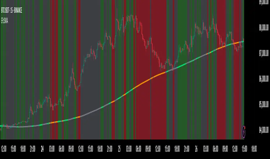
[GYTS-CE] Market Regime Detector🧊 Market Regime Detector (Community Edition)
🌸 Part of GoemonYae Trading System (GYTS) 🌸
🌸 --------- INTRODUCTION --------- 🌸
💮 What is the Market Regime Detector?
The Market Regime Detector is an advanced, consensus-based indicator that identifies the current market state to increase the probability of profitable trades. By distinguishing between trending (bullish or bearish) and cyclic (range-bound) market conditions, this detector helps you select appropriate tactics for different environments. Instead of forcing a single strategy across all market conditions, our detector allows you to adapt your approach based on real-time market behaviour.
💮 The Importance of Market Regimes
Markets constantly shift between different behavioural states or "regimes":
• Bullish trending markets - characterised by sustained upward price movement
• Bearish trending markets - characterised by sustained downward price movement
• Cyclic markets - characterised by range-bound, oscillating behaviour
Each regime requires fundamentally different trading approaches. Trend-following strategies excel in trending markets but fail in cyclic ones, while mean-reversion strategies shine in cyclic markets but underperform in trending conditions. Detecting these regimes is essential for successful trading, which is why we've developed the Market Regime Detector to accurately identify market states using complementary detection methods.
🌸 --------- KEY FEATURES --------- 🌸
💮 Consensus-Based Detection
Rather than relying on a single method, our detector employs two complementary detection methodologies that analyse different aspects of market behaviour:
• Dominant Cycle Average (DCA) - analyzes price movement relative to its lookback period, a proxy for the dominant cycle
• Volatility Channel - examines price behaviour within adaptive volatility bands
These diverse perspectives are synthesised into a robust consensus that minimises false signals while maintaining responsiveness to genuine regime changes.
💮 Dominant Cycle Framework
The Market Regime Detector uses the concept of dominant cycles to establish a reference framework. You can input the dominant cycle period that best represents the natural rhythm of your market, providing a stable foundation for regime detection across different timeframes.
💮 Intuitive Parameter System
We've distilled complex technical parameters into intuitive controls that traders can easily understand:
• Adaptability - how quickly the detector responds to changing market conditions
• Sensitivity - how readily the detector identifies transitions between regimes
• Consensus requirement - how much agreement is needed among detection methods
This approach makes the detector accessible to traders of all experience levels while preserving the power of the underlying algorithms.
💮 Visual Market Feedback
The detector provides clear visual feedback about the current market regime through:
• Colour-coded chart backgrounds (purple shades for bullish, pink for bearish, yellow for cyclic)
• Colour-coded price bars
• Strength indicators showing the degree of consensus
• Customizable colour schemes to match your preferences or trading system
💮 Integration in the GYTS suite
The Market Regime Detector is compatible with the GYTS Suite , i.e. it passes the regime into the 🎼 Order Orchestrator where you can set how to trade the trending and cyclic regime.
🌸 --------- CONFIGURATION SETTINGS --------- 🌸
💮 Adaptability
Controls how quickly the Market Regime detector adapts to changing market conditions. You can see it as a low-frequency, long-term change parameter:
Very Low: Very slow adaptation, most stable but may miss regime changes
Low: Slower adaptation, more stability but less responsiveness
Normal: Balanced between stability and responsiveness
High: Faster adaptation, more responsive but less stable
Very High: Very fast adaptation, highly responsive but may generate false signals
This setting affects lookback periods and filter parameters across all detection methods.
💮 Sensitivity
Controls how sensitive the detector is to market regime transitions. This acts as a high-frequency, short-term change parameter:
Very Low: Requires substantial evidence to identify a regime change
Low: Less sensitive, reduces false signals but may miss some transitions
Normal: Balanced sensitivity suitable for most markets
High: More sensitive, detects subtle regime changes but may have more noise
Very High: Very sensitive, detects minor fluctuations but may produce frequent changes
This setting affects thresholds for regime detection across all methods.
💮 Dominant Cycle Period
This parameter allows you to specify the market's natural rhythm in bars. This represents a complete market cycle (up and down movement). Finding the right value for your specific market and timeframe might require some experimentation, but it's a crucial parameter that helps the detector accurately identify regime changes. Most of the times the cycle is between 20 and 40 bars.
💮 Consensus Mode
Determines how the signals from both detection methods are combined to produce the final market regime:
• Any Method (OR) : Signals bullish/bearish if either method detects that regime. If methods conflict (one bullish, one bearish), the stronger signal wins. More sensitive, catches more regime changes but may produce more false signals.
• All Methods (AND) : Signals only when both methods agree on the regime. More conservative, reduces false signals but might miss some legitimate regime changes.
• Weighted Decision : Balances both methods with equal weighting. Provides a middle ground between sensitivity and stability.
Each mode also calculates a continuous regime strength value that's used for colour intensity in the 'unconstrained' display mode.
💮 Display Mode
Choose how to display the market regime colours:
• Unconstrained regime: Shows the regime strength as a continuous gradient. This provides more nuanced visualisation where the intensity of the colour indicates the strength of the trend.
• Consensus only: Shows only the final consensus regime with fixed colours based on the detected regime type.
The background and bar colours will change to indicate the current market regime:
• Purple shades: Bullish trending market (darker purple indicates stronger bullish trend)
• Pink shades: Bearish trending market (darker pink indicates stronger bearish trend)
• Yellow: Cyclic (range-bound) market
💮 Custom Colour Options
The Market Regime Detector allows you to customize the colour scheme to match your personal preferences or to coordinate with other indicators:
• Use custom colours: Toggle to enable your own colour choices instead of the default scheme
• Transparency: Adjust the transparency level of all regime colours
• Bullish colours: Define custom colours for strong, medium, weak, and very weak bullish trends
• Bearish colours: Define custom colours for strong, medium, weak, and very weak bearish trends
• Cyclic colour: Define a custom colour for cyclic (range-bound) market conditions
🌸 --------- DETECTION METHODS --------- 🌸
💮 Dominant Cycle Average (DCA)
The Dominant Cycle Average method forms a key part of our detection system:
1. Theoretical Foundation :
The DCA method builds on cycle analysis and the observation that in trending markets, price consistently remains on one side of a moving average calculated using the dominant cycle period. In contrast, during cyclic markets, price oscillates around this average.
2. Calculation Process :
• We calculate a Simple Moving Average (SMA) using the specified lookback period - a proxy for the dominant cycle period
• We then analyse the proportion of time that price spends above or below this SMA over a lookback window. The theory is that the price should cross the SMA each half cycle, assuming that the dominant cycle period is correct and price follows a sinusoid.
• This lookback window is adaptive, scaling with the dominant cycle period (controlled by the Adaptability setting)
• The different values are standardised and normalised to possess more resolving power and to be more robust to noise.
3. Regime Classification :
• When the normalised proportion exceeds a positive threshold (determined by Sensitivity setting), the market is classified as bullish trending
• When it falls below a negative threshold, the market is classified as bearish trending
• When the proportion remains between these thresholds, the market is classified as cyclic
💮 Volatility Channel
The Volatility Channel method complements the DCA method by focusing on price movement relative to adaptive volatility bands:
1. Theoretical Foundation :
This method is based on the observation that trending markets tend to sustain movement outside of normal volatility ranges, while cyclic markets tend to remain contained within these ranges. By creating adaptive bands that adjust to current market volatility, we can detect when price behaviour indicates a trending or cyclic regime.
2. Calculation Process :
• We first calculate a smooth base channel center using a low pass filter, creating a noise-reduced centreline for price
• True Range (TR) is used to measure market volatility, which is then smoothed and scaled by the deviation factor (controlled by Sensitivity)
• Upper and lower bands are created by adding and subtracting this scaled volatility from the centreline
• Price is smoothed using an adaptive A2RMA filter, which has a very flat and stable behaviour, to reduce noise while preserving trend characteristics
• The position of this smoothed price relative to the bands is continuously monitored
3. Regime Classification :
• When smoothed price moves above the upper band, the market is classified as bullish trending
• When smoothed price moves below the lower band, the market is classified as bearish trending
• When price remains between the bands, the market is classified as cyclic
• The magnitude of price's excursion beyond the bands is used to determine trend strength
4. Adaptive Behaviour :
• The smoothing periods and deviation calculations automatically adjust based on the Adaptability setting
• The measured volatility is calculated over a period proportional to the dominant cycle, ensuring the detector works across different timeframes
• Both the center line and the bands adapt dynamically to changing market conditions, making the detector responsive yet stable
This method provides a unique perspective that complements the DCA approach, with the consensus mechanism synthesising insights from both methods.
🌸 --------- USAGE GUIDE --------- 🌸
💮 Starting with Default Settings
The default settings (Normal for Adaptability and Sensitivity, Weighted Decision for Consensus Mode) provide a balanced starting point suitable for most markets and timeframes. Begin by observing how these settings identify regimes in your preferred instruments.
💮 Finding the Optimal Dominant Cycle
The dominant cycle period is a critical parameter. Here are some approaches to finding an appropriate value:
• Start with typical values, usually something around 25 works well
• Visually identify the average distance between significant peaks and troughs
• Experiment with different values and observe which provides the most stable regime identification
• Consider using cycle-finding indicators to help identify the natural rhythm of your market
💮 Adjusting Parameters
• If you notice too many regime changes → Decrease Sensitivity or increase Consensus requirement
• If regime changes seem delayed → Increase Adaptability
• If a trending regime is not detected, the market is automatically assigned to be in a cyclic state
• If you want to see more nuanced regime transitions → Try the "unconstrained" display mode (note that this will not affect the output to other indicators)
💮 Trading Applications
Regime-Specific Strategies:
• Bullish Trending Regime - Use trend-following strategies, trail stops wider, focus on breakouts, consider holding positions longer, and emphasize buying dips
• Bearish Trending Regime - Consider shorts, tighter stops, focus on breakdown points, sell rallies, implement downside protection, and reduce position sizes
• Cyclic Regime - Apply mean-reversion strategies, trade range boundaries, apply oscillators, target definable support/resistance levels, and use profit-taking at extremes
Strategy Switching:
Create a set of rules for each market regime and switch between them based on the detector's signal. This approach can significantly improve performance compared to applying a single strategy across all market conditions.
GYTS Suite Integration:
• In the GYTS 🎼 Order Orchestrator, select the '🔗 STREAM-int 🧊 Market Regime' as the market regime source
• Note that the consensus output (i.e. not the "unconstrained" display) will be used in this stream
• Create different strategies for trending (bullish/bearish) and cyclic regimes. The GYTS 🎼 Order Orchestrator is specifically made for this.
• The output stream is actually very simple, and can possibly be used in indicators and strategies as well. It outputs 1 for bullish, -1 for bearish and 0 for cyclic regime.
🌸 --------- FINAL NOTES --------- 🌸
💮 Development Philosophy
The Market Regime Detector has been developed with several key principles in mind:
1. Robustness - The detection methods have been rigorously tested across diverse markets and timeframes to ensure reliable performance.
2. Adaptability - The detector automatically adjusts to changing market conditions, requiring minimal manual intervention.
3. Complementarity - Each detection method provides a unique perspective, with the collective consensus being more reliable than any individual method.
4. Intuitiveness - Complex technical parameters have been abstracted into easily understood controls.
💮 Ongoing Refinement
The Market Regime Detector is under continuous development. We regularly:
• Fine-tune parameters based on expanded market data
• Research and integrate new detection methodologies
• Optimise computational efficiency for real-time analysis
Your feedback and suggestions are very important in this ongoing refinement process!
Dual SuperTrend w VIX Filter - Strategy [presentTrading]Hey everyone! Haven't been here for a long time. Been so busy again in the past 2 months. I recently started working on analyzing the combination of trend strategy and VIX, but didn't get outstanding results after a few tries. Sharing this tool with all of you in case you have better insights.
█ Introduction and How it is Different
The Dual SuperTrend with VIX Filter Strategy combines traditional trend following with market volatility analysis. Unlike conventional SuperTrend strategies that focus solely on price action, this experimental system incorporates VIX (Volatility Index) as an adaptive filter to create a more context-aware trading approach. By analyzing where current volatility stands relative to historical norms, the strategy adjusts to different market environments rather than applying uniform logic across all conditions.
BTCUSD 6hr Long Short Performance
█ Strategy, How it Works: Detailed Explanation
🔶 Dual SuperTrend Core
The strategy uses two SuperTrend indicators with different sensitivity settings:
- SuperTrend 1: Length = 13, Multiplier = 3.5
- SuperTrend 2: Length = 8, Multiplier = 5.0
The SuperTrend calculation follows this process:
1. ATR = Average of max(High-Low, |High-PreviousClose|, |Low-PreviousClose|) over 'length' periods
2. UpperBand = (High+Low)/2 - (Multiplier * ATR)
3. LowerBand = (High+Low)/2 + (Multiplier * ATR)
Trend direction is determined by:
- If Close > previous LowerBand, Trend = Bullish (1)
- If Close < previous UpperBand, Trend = Bearish (-1)
- Otherwise, Trend = previous Trend
🔶 VIX Analysis Framework
The core innovation lies in the VIX analysis system:
1. Statistical Analysis:
- VIX Mean = SMA(VIX, 252)
- VIX Standard Deviation = StdDev(VIX, 252)
- VIX Z-Score = (Current VIX - VIX Mean) / VIX StdDev
2. **Volatility Bands:
- Upper Band 1 = VIX Mean + (2 * VIX StdDev)
- Upper Band 2 = VIX Mean + (3 * VIX StdDev)
- Lower Band 1 = VIX Mean - (2 * VIX StdDev)
- Lower Band 2 = VIX Mean - (3 * VIX StdDev)
3. Volatility Regimes:
- "Very Low Volatility": VIX < Lower Band 1
- "Low Volatility": Lower Band 1 ≤ VIX < Mean
- "Normal Volatility": Mean ≤ VIX < Upper Band 1
- "High Volatility": Upper Band 1 ≤ VIX < Upper Band 2
- "Extreme Volatility": VIX ≥ Upper Band 2
4. VIX Trend Detection:
- VIX EMA = EMA(VIX, 10)
- VIX Rising = VIX > VIX EMA
- VIX Falling = VIX < VIX EMA
Local performance:
🔶 Entry Logic Integration
The strategy combines trend signals with volatility filtering:
Long Entry Condition:
- Both SuperTrend 1 AND SuperTrend 2 must be bullish (trend = 1)
- AND selected VIX filter condition must be satisfied
Short Entry Condition:
- Both SuperTrend 1 AND SuperTrend 2 must be bearish (trend = -1)
- AND selected VIX filter condition must be satisfied
Available VIX filter rules include:
- "Below Mean + SD": VIX < Lower Band 1
- "Below Mean": VIX < VIX Mean
- "Above Mean": VIX > VIX Mean
- "Above Mean + SD": VIX > Upper Band 1
- "Falling VIX": VIX < VIX EMA
- "Rising VIX": VIX > VIX EMA
- "Any": No VIX filtering
█ Trade Direction
The strategy allows testing in three modes:
1. **Long Only:** Test volatility effects on uptrends only
2. **Short Only:** Examine volatility's impact on downtrends only
3. **Both (Default):** Compare how volatility affects both trend directions
This enables comparative analysis of how volatility regimes impact bullish versus bearish markets differently.
█ Usage
Use this strategy as an experimental framework:
1. Form a hypothesis about how volatility affects trend reliability
2. Configure VIX filters to test your specific hypothesis
3. Analyze performance across different volatility regimes
4. Compare results between uptrends and downtrends
5. Refine your volatility filtering approach based on results
6. Share your findings with the trading community
This framework allows you to investigate questions like:
- Are uptrends more reliable during rising or falling volatility?
- Do downtrends perform better when volatility is above or below its historical average?
- Should different volatility filters be applied to long vs. short positions?
█ Default Settings
The default settings serve as a starting point for exploration:
SuperTrend Parameters:
- SuperTrend 1 (Length=13, Multiplier=3.5): More responsive to trend changes
- SuperTrend 2 (Length=8, Multiplier=5.0): More selective filter requiring stronger trends
VIX Analysis Settings:
- Lookback Period = 252: Establishes a full market cycle for volatility context
- Standard Deviation Bands = 2 and 3 SD: Creates statistically significant regime boundaries
- VIX Trend Period = 10: Balances responsiveness with noise reduction
Default VIX Filter Selection:
- Long Entry: "Above Mean" - Tests if uptrends perform better during above-average volatility
- Short Entry: "Rising VIX" - Tests if downtrends accelerate when volatility is increasing
Feel Free to share your insight below!!!

Gradient Trend Filter [ChartPrime]The Gradient Trend Filter is a dynamic trend analysis tool that combines a noise-filtered trend detection system with a color-gradient cloud. It provides traders with a visual representation of trend strength, momentum shifts, and potential reversals.
⯁ KEY FEATURES
Trend Noise Filtering
Uses an advanced smoothing function to filter market noise and produce a more reliable trend representation.
// Noise filter function
noise_filter(src, length) =>
alpha = 2 / (length + 1)
nf_1 = 0.0
nf_2 = 0.0
nf_3 = 0.0
nf_1 := (alpha * src) + ((1 - alpha) * nz(nf_1 ))
nf_2 := (alpha * nf_1) + ((1 - alpha) * nz(nf_2 ))
nf_3 := (alpha * nf_2) + ((1 - alpha) * nz(nf_3 ))
nf_3 // Final output with three-stage smoothing
Color-Based Trend Visualization
The mid-line changes color based on trend direction—green for uptrends and red for downtrends—making it easy to identify trends at a glance.
Orange diamond markers appear when a trend shift is confirmed, providing actionable signals for traders.
Gradient Color Trend Cloud
A cloud around the base trend line that dynamically changes color, often signaling trend shifts ahead of the main trend line.
When in a downtrend, if the cloud starts turning green, it suggests weakening bearish momentum or an upcoming bullish reversal. Conversely, when in an uptrend, a red cloud indicates potential trend weakening or a bearish reversal.
Multi-Layered Trend Bands
The cloud consists of multiple bands, offering a range of support and resistance zones that traders can use for confluence in decision-making.
⯁ HOW TO USE
Identify Trend Strength & Reversals
Use the mid-line and cloud color changes to assess the strength of a trend and spot early signs of reversals.
Monitor Momentum Shifts
Watch for gradient cloud color shifts before the trend line changes color, as this can indicate early weakening or strengthening of momentum.
Act on Trend Shift Markers
Use the orange diamonds as confirmation of trend shifts and potential trade entry or exit points.
Utilize Cloud Bands as Support/Resistance
The outer bands of the cloud act as dynamic support and resistance, helping traders refine their stop-loss and take-profit placements.
⯁ CONCLUSION
The Gradient Trend Filter is an advanced trend detection tool designed for traders looking to anticipate trend shifts with greater precision. By integrating a noise-filtered trend line with a gradient-based trend cloud, this indicator enhances traders' ability to navigate market trends effectively.
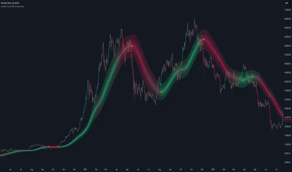
[GYTS] Filters ToolkitFilters Toolkit indicator
🌸 Part of GoemonYae Trading System (GYTS) 🌸
🌸 --------- 1. INTRODUCTION --------- 🌸
💮 Overview
The GYTS Filters Toolkit indicator is an advanced, interactive interface built atop the high‐performance, curated functions provided by the FiltersToolkit library . It allows traders to experiment with different combinations of filtering methods -— from smoothing low-pass filters to aggressive detrenders. With this toolkit, you can build custom indicators tailored to your specific trading strategy, whether you're looking for trend following, mean reversion, or cycle identification approaches.
🌸 --------- 2. FILTER METHODS AND TYPES --------- 🌸
💮 Filter categories
The available filters fall into four main categories, each marked with a distinct symbol:
🌗 Low Pass Filters (Smoothers)
These filters attenuate high-frequency components (noise) while allowing low-frequency components (trends) to pass through. Examples include:
Ultimate Smoother
Super Smoother (2-pole and 3-pole variants)
MESA Adaptive Moving Average (MAMA) and Following Adaptive Moving Average (FAMA)
BiQuad Low Pass Filter
ADXvma (Adaptive Directional Volatility Moving Average)
A2RMA (Adaptive Autonomous Recursive Moving Average)
Low pass filters are displayed on the price chart by default, as they follow the overall price movement. If they are combined with a high-pass or bandpass filter, they will be displayed in the subgraph.
🌓 High Pass Filters (Detrenders)
These filters do the opposite of low pass filters - they remove low-frequency components (trends) while allowing high-frequency components to pass through. Examples include:
Butterworth High Pass Filter
BiQuad High Pass Filter
High pass filters are displayed as oscillators in the subgraph below the price chart, as they fluctuate around a zero line.
🌑 Band Pass Filters (Cycle Isolators)
These filters combine aspects of both low and high pass filters, isolating specific frequency ranges while attenuating both higher and lower frequencies. Examples include:
Ehlers Bandpass Filter
Cyber Cycle
Relative Vigor Index (RVI)
BiQuad Bandpass Filter
Band pass filters are also displayed as oscillators in a separate panel.
🔮 Predictive Filter
Voss Predictive Filter: A special filter that attempts to predict future values of band-limited signals (only to be used as post-filter). Keep its prediction horizon short (1–3 bars) for reasonable accuracy.
Note that the the library contains elaborate documentation and source material of each filter.
🌸 --------- 3. INDICATOR FEATURES --------- 🌸
💮 Multi-filter configuration
One of the most powerful aspects of this indicator is the ability to configure multiple filters. compare them and observe their combined effects. There are four primary filters, each with its own parameter settings.
💮 Post-filtering
Process a filter’s output through an additional filter by enabling the post-filter option. This creates a filter chain where the output of one filter becomes the input to another. Some powerful combinations include:
Ultimate Smoother → MAMA: Creates an adaptive smoothing effect that responds well to market changes, good for trend-following strategies
Butterworth → Super Smoother → Butterworth: Produces a well-behaved oscillator with minimal phase distortion, John Ehlers also calls a "roofing filter". Great for identifying overbought/oversold conditions with minimal lag.
A bandpass filter → Voss Prediction filter: Attempts to predict future movements of cyclical components, handy to find peaks and troughs of the market cycle.
💮 Aggregate filters
Arguably the coolest feature: aggregating filters allow you to combine multiple filters with different weights. Important notes about aggregation:
You can only aggregate filters that appear on the same chart (price chart or oscillator panel).
The weights are automatically normalised, so only their relative values matter
Setting a weight to 0 (zero) excludes that filter from the aggregation
Filters don't need to be visibly displayed to be included in aggregation
💮 Rich visualisation & alerts
The indicator intelligently determines whether a filter is displayed on the price chart or in the subgraph (as an oscillator) based on its characteristics.
Dynamic colour palettes, adjustable line widths, transparency, and custom fill between any of enabled filters or between oscillators and the zero-line.
A clear legend showing which filters are active and how they're configured
Alerts for direction changes and crossovers of all filters
🌸 --------- 4. ACKNOWLEDGEMENTS --------- 🌸
This toolkit builds on the work of numerous pioneers in technical analysis and digital signal processing:
John Ehlers, whose groundbreaking research forms the foundation of many filters.
Robert Bristow-Johnson for the BiQuad filter formulations.
The TradingView community, especially @The_Peaceful_Lizard, @alexgrover, and others mentioned in the code of the library.
Everyone who has provided feedback, testing and support!
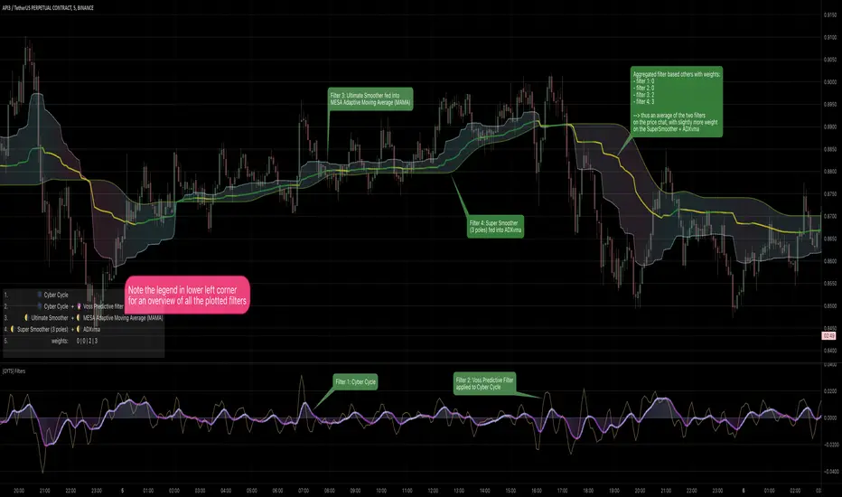
[GYTS] FiltersToolkit LibraryFiltersToolkit Library
🌸 Part of GoemonYae Trading System (GYTS) 🌸
🌸 --------- 1. INTRODUCTION --------- 🌸
💮 What Does This Library Contain?
This library is a curated collection of high-performance digital signal processing (DSP) filters and auxiliary functions designed specifically for financial time series analysis. It includes a shortlist of our favourite and best performing filters — each rigorously tested and selected for their responsiveness, minimal lag and robustness in diverse market conditions. These tools form an integral part of the GoemonYae Trading System (GYTS), chosen for their unique characteristics in handling market data.
The library contains two main categories:
1. Smoothing filters (low-pass filters and moving averages) for e.g. denoising, trend following
2. Detrending tools (high-pass and band-pass filters, known as "oscillators") for e.g. mean reversion
This collection is finely tuned for practical trading applications and is therefore not meant to be exhaustive. However, will continue to expand as we discover and validate new filtering techniques. I welcome collaboration and suggestions for novel approaches.
🌸 ——— 2. ADDED VALUE ——— 🌸
💮 Unified syntax and comprehensive documentation
The FiltersToolkit Library brings together a wide array of valuable filters under a unified, intuitive syntax. Each function is thoroughly documented, with clear explanations and academic sources that underline the mathematical rigour behind the methods. This level of documentation not only facilitates integration into trading strategies but also helps underlying the underlying concepts and rationale.
💮 Optimised performance and readability
The code prioritizes computational efficiency while maintaining readability. Key optimizations include:
- Minimizing redundant calculations in recursive filters
- Smart coefficient caching
- Efficient state management
- Vectorized operations where applicable
💮 Enhanced functionality and flexibility
Some filters in this library introduce extended functionality beyond the original publications. For instance, the MESA Adaptive Moving Average (MAMA) and Ehlers’ Combined Bandpass Filter incorporate multiple variations found in the literature, thereby providing traders with flexible tools that can be fine-tuned to different market conditions.
🌸 ——— 3. THE FILTERS ——— 🌸
💮 Hilbert Transform Function
This function implements the Hilbert Transform as utilised by John Ehlers. It converts a real-valued time series into its analytic signal, enabling the extraction of instantaneous phase and frequency information—an essential step in adaptive filtering.
Source: John Ehlers - "Rocket Science for Traders" (2001), "TASC 2001 V. 19:9", "Cybernetic Analysis for Stocks and Futures" (2004)
💮 Homodyne Discriminator
By leveraging the Hilbert Transform, this function computes the dominant cycle period through a Homodyne Discriminator. It extracts the in-phase and quadrature components of the signal, facilitating a robust estimation of the underlying cycle characteristics.
Source: John Ehlers - "Rocket Science for Traders" (2001), "TASC 2001 V. 19:9", "Cybernetic Analysis for Stocks and Futures" (2004)
💮 MESA Adaptive Moving Average (MAMA)
An advanced dual-stage adaptive moving average, this function outputs both the MAMA and its companion FAMA. It combines adaptive alpha computation with elements from Kaufman’s Adaptive Moving Average (KAMA) to provide a responsive and reliable trend indicator.
Source: John Ehlers - "Rocket Science for Traders" (2001), "TASC 2001 V. 19:9", "Cybernetic Analysis for Stocks and Futures" (2004)
💮 BiQuad Filters
A family of second-order recursive filters offering exceptional control over frequency response:
- High-pass filter for detrending
- Low-pass filter for smooth trend following
- Band-pass filter for cycle isolation
The quality factor (Q) parameter allows fine-tuning of the resonance characteristics, making these filters highly adaptable to different market conditions.
Source: Robert Bristow-Johnson's Audio EQ Cookbook, implemented by @The_Peaceful_Lizard
💮 Relative Vigor Index (RVI)
This filter evaluates the strength of a trend by comparing the closing price to the trading range. Operating similarly to a band-pass filter, the RVI provides insights into market momentum and potential reversals.
Source: John Ehlers – “Cybernetic Analysis for Stocks and Futures” (2004)
💮 Cyber Cycle
The Cyber Cycle filter emphasises market cycles by smoothing out noise and highlighting the dominant cyclical behaviour. It is particularly useful for detecting trend reversals and cyclical patterns in the price data.
Source: John Ehlers – “Cybernetic Analysis for Stocks and Futures” (2004)
💮 Butterworth High Pass Filter
Inspired by the classical Butterworth design, this filter achieves a maximally flat magnitude response in the passband while effectively removing low-frequency trends. Its design minimises phase distortion, which is vital for accurate signal interpretation.
Source: John Ehlers – “Cybernetic Analysis for Stocks and Futures” (2004)
💮 2-Pole SuperSmoother
Employing a two-pole design, the SuperSmoother filter reduces high-frequency noise with minimal lag. It is engineered to preserve trend integrity while offering a smooth output even in noisy market conditions.
Source: John Ehlers – “Cybernetic Analysis for Stocks and Futures” (2004)
💮 3-Pole SuperSmoother
An extension of the 2-pole design, the 3-pole SuperSmoother further attenuates high-frequency noise. Its additional pole delivers enhanced smoothing at the cost of slightly increased lag.
Source: John Ehlers – “Cybernetic Analysis for Stocks and Futures” (2004)
💮 Adaptive Directional Volatility Moving Average (ADXVma)
This adaptive moving average adjusts its smoothing factor based on directional volatility. By combining true range and directional movement measurements, it remains exceptionally flat during ranging markets and responsive during directional moves.
Source: Various implementations across platforms, unified and optimized
💮 Ehlers Combined Bandpass Filter with Automated Gain Control (AGC)
This sophisticated filter merges a highpass pre-processing stage with a bandpass filter. An integrated Automated Gain Control normalises the output to a consistent range, while offering both regular and truncated recursive formulations to manage lag.
Source: John F. Ehlers – “Truncated Indicators” (2020), “Cycle Analytics for Traders” (2013)
💮 Voss Predictive Filter
A forward-looking filter that predicts future values of a band-limited signal in real time. By utilising multiple time-delayed feedback terms, it provides anticipatory coupling and delivers a short-term predictive signal.
Source: John Ehlers - "A Peek Into The Future" (TASC 2019-08)
💮 Adaptive Autonomous Recursive Moving Average (A2RMA)
This filter dynamically adjusts its smoothing through an adaptive mechanism based on an efficiency ratio and a dynamic threshold. A double application of an adaptive moving average ensures both responsiveness and stability in volatile and ranging markets alike. Very flat response when properly tuned.
Source: @alexgrover (2019)
💮 Ultimate Smoother (2-Pole)
The Ultimate Smoother filter is engineered to achieve near-zero lag in its passband by subtracting a high-pass response from an all-pass response. This creates a filter that maintains signal fidelity at low frequencies while effectively filtering higher frequencies at the expense of slight overshooting.
Source: John Ehlers - TASC 2024-04 "The Ultimate Smoother"
Note: This library is actively maintained and enhanced. Suggestions for additional filters or improvements are welcome through the usual channels. The source code contains a list of tested filters that did not make it into the curated collection.
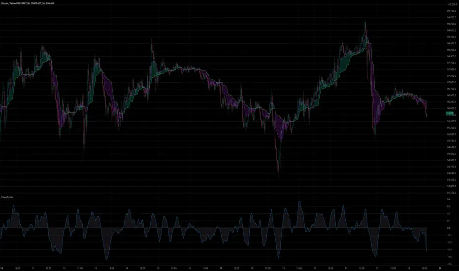
PaddingThe Padding library is a comprehensive and flexible toolkit designed to extend time series data within TradingView, making it an indispensable resource for advanced signal processing tasks such as FFT, filtering, convolution, and wavelet analysis. At its core, the library addresses the common challenge of edge effects by "padding" your data—that is, by appending additional data points beyond the natural boundaries of your original dataset. This extension not only mitigates the distortions that can occur at the endpoints but also helps to maintain the integrity of various transformations and calculations performed on the series. The library accomplishes this while preserving the ordering of your data, ensuring that the most recent point always resides at index 0.
Central to the functionality of this library are two key enumerations: Direction and PaddingType. The Direction enum determines where the padding will be applied. You can choose to extend the data in the forward direction (ahead of the current values), in the backward direction (behind the current values), or in both directions simultaneously. The PaddingType enum defines the specific method used for extending the data. The library supports several methods—including symmetric, reflect, periodic, antisymmetric, antireflect, smooth, constant, and zero padding—each of which has been implemented to suit different analytical scenarios. For instance, symmetric padding mirrors the original data across its boundaries, while reflect padding continues the trend by reflecting around endpoint values. Periodic padding repeats the data, and antisymmetric padding mirrors the data with alternating signs to counterbalance it. The antireflect and smooth methods take into account the derivatives of your data, thereby extending the series in a way that preserves or smoothly continues these derivative values. Constant and zero padding simply extend the series using fixed endpoint values or zeros. Together, these enums allow you to fine-tune how your data is extended, ensuring that the padding method aligns with the specific requirements of your analysis.
The library is designed to work with both single variable inputs and array inputs. When using array-based methods—particularly with the antireflect and smooth padding types—please note that the implementation intentionally discards the last data point as a result of the delta computation process. This behavior is an important consideration when integrating the library into your TradingView studies, as it affects the overall data length of the padded series. Despite this, the library’s structure and documentation make it straightforward to incorporate into your existing scripts. You simply provide your data source, define the length of your data window, and select the desired padding type and direction, along with any optional parameters to control the extent of the padding (using both_period, forward_period, or backward_period).
In practical application, the Padding library enables you to extend historical data beyond its original range in a controlled and predictable manner. This is particularly useful when preparing datasets for further signal processing, as it helps to reduce artifacts that can otherwise compromise the results of your analytical routines. Whether you are an experienced Pine Script developer or a trader exploring advanced data analysis techniques, this library offers a robust solution that enhances the reliability and accuracy of your studies by ensuring your algorithms operate on a more complete and well-prepared dataset.
Library "Padding"
A comprehensive library for padding time series data with various methods. Supports both single variable and array inputs, with flexible padding directions and periods. Designed for signal processing applications including FFT, filtering, convolution, and wavelets. All methods maintain data ordering with most recent point at index 0.
symmetric(source, series_length, direction, both_period, forward_period, backward_period)
Applies symmetric padding by mirroring the input data across boundaries
Parameters:
source (float) : Input value to pad from
series_length (int) : Length of the data window
direction (series Direction) : Direction to apply padding
both_period (int) : Optional - periods to pad in both directions. Overrides forward_period and backward_period if specified
forward_period (int) : Optional - periods to pad forward. Defaults to series_length if not specified
backward_period (int) : Optional - periods to pad backward. Defaults to series_length if not specified
Returns: Array ordered with most recent point at index 0, containing original data with symmetric padding applied
method symmetric(source, direction, both_period, forward_period, backward_period)
Applies symmetric padding to an array by mirroring the data across boundaries
Namespace types: array
Parameters:
source (array) : Array of values to pad
direction (series Direction) : Direction to apply padding
both_period (int) : Optional - periods to pad in both directions. Overrides forward_period and backward_period if specified
forward_period (int) : Optional - periods to pad forward. Defaults to array length if not specified
backward_period (int) : Optional - periods to pad backward. Defaults to array length if not specified
Returns: Array ordered with most recent point at index 0, containing original data with symmetric padding applied
reflect(source, series_length, direction, both_period, forward_period, backward_period)
Applies reflect padding by continuing trends through reflection around endpoint values
Parameters:
source (float) : Input value to pad from
series_length (int) : Length of the data window
direction (series Direction) : Direction to apply padding
both_period (int) : Optional - periods to pad in both directions. Overrides forward_period and backward_period if specified
forward_period (int) : Optional - periods to pad forward. Defaults to series_length if not specified
backward_period (int) : Optional - periods to pad backward. Defaults to series_length if not specified
Returns: Array ordered with most recent point at index 0, containing original data with reflect padding applied
method reflect(source, direction, both_period, forward_period, backward_period)
Applies reflect padding to an array by continuing trends through reflection around endpoint values
Namespace types: array
Parameters:
source (array) : Array of values to pad
direction (series Direction) : Direction to apply padding
both_period (int) : Optional - periods to pad in both directions. Overrides forward_period and backward_period if specified
forward_period (int) : Optional - periods to pad forward. Defaults to array length if not specified
backward_period (int) : Optional - periods to pad backward. Defaults to array length if not specified
Returns: Array ordered with most recent point at index 0, containing original data with reflect padding applied
periodic(source, series_length, direction, both_period, forward_period, backward_period)
Applies periodic padding by repeating the input data
Parameters:
source (float) : Input value to pad from
series_length (int) : Length of the data window
direction (series Direction) : Direction to apply padding
both_period (int) : Optional - periods to pad in both directions. Overrides forward_period and backward_period if specified
forward_period (int) : Optional - periods to pad forward. Defaults to series_length if not specified
backward_period (int) : Optional - periods to pad backward. Defaults to series_length if not specified
Returns: Array ordered with most recent point at index 0, containing original data with periodic padding applied
method periodic(source, direction, both_period, forward_period, backward_period)
Applies periodic padding to an array by repeating the data
Namespace types: array
Parameters:
source (array) : Array of values to pad
direction (series Direction) : Direction to apply padding
both_period (int) : Optional - periods to pad in both directions. Overrides forward_period and backward_period if specified
forward_period (int) : Optional - periods to pad forward. Defaults to array length if not specified
backward_period (int) : Optional - periods to pad backward. Defaults to array length if not specified
Returns: Array ordered with most recent point at index 0, containing original data with periodic padding applied
antisymmetric(source, series_length, direction, both_period, forward_period, backward_period)
Applies antisymmetric padding by mirroring data and alternating signs
Parameters:
source (float) : Input value to pad from
series_length (int) : Length of the data window
direction (series Direction) : Direction to apply padding
both_period (int) : Optional - periods to pad in both directions. Overrides forward_period and backward_period if specified
forward_period (int) : Optional - periods to pad forward. Defaults to series_length if not specified
backward_period (int) : Optional - periods to pad backward. Defaults to series_length if not specified
Returns: Array ordered with most recent point at index 0, containing original data with antisymmetric padding applied
method antisymmetric(source, direction, both_period, forward_period, backward_period)
Applies antisymmetric padding to an array by mirroring data and alternating signs
Namespace types: array
Parameters:
source (array) : Array of values to pad
direction (series Direction) : Direction to apply padding
both_period (int) : Optional - periods to pad in both directions. Overrides forward_period and backward_period if specified
forward_period (int) : Optional - periods to pad forward. Defaults to array length if not specified
backward_period (int) : Optional - periods to pad backward. Defaults to array length if not specified
Returns: Array ordered with most recent point at index 0, containing original data with antisymmetric padding applied
antireflect(source, series_length, direction, both_period, forward_period, backward_period)
Applies antireflect padding by reflecting around endpoints while preserving derivatives
Parameters:
source (float) : Input value to pad from
series_length (int) : Length of the data window
direction (series Direction) : Direction to apply padding
both_period (int) : Optional - periods to pad in both directions. Overrides forward_period and backward_period if specified
forward_period (int) : Optional - periods to pad forward. Defaults to series_length if not specified
backward_period (int) : Optional - periods to pad backward. Defaults to series_length if not specified
Returns: Array ordered with most recent point at index 0, containing original data with antireflect padding applied
method antireflect(source, direction, both_period, forward_period, backward_period)
Applies antireflect padding to an array by reflecting around endpoints while preserving derivatives
Namespace types: array
Parameters:
source (array) : Array of values to pad
direction (series Direction) : Direction to apply padding
both_period (int) : Optional - periods to pad in both directions. Overrides forward_period and backward_period if specified
forward_period (int) : Optional - periods to pad forward. Defaults to array length if not specified
backward_period (int) : Optional - periods to pad backward. Defaults to array length if not specified
Returns: Array ordered with most recent point at index 0, containing original data with antireflect padding applied. Note: Last data point is lost when using array input
smooth(source, series_length, direction, both_period, forward_period, backward_period)
Applies smooth padding by extending with constant derivatives from endpoints
Parameters:
source (float) : Input value to pad from
series_length (int) : Length of the data window
direction (series Direction) : Direction to apply padding
both_period (int) : Optional - periods to pad in both directions. Overrides forward_period and backward_period if specified
forward_period (int) : Optional - periods to pad forward. Defaults to series_length if not specified
backward_period (int) : Optional - periods to pad backward. Defaults to series_length if not specified
Returns: Array ordered with most recent point at index 0, containing original data with smooth padding applied
method smooth(source, direction, both_period, forward_period, backward_period)
Applies smooth padding to an array by extending with constant derivatives from endpoints
Namespace types: array
Parameters:
source (array) : Array of values to pad
direction (series Direction) : Direction to apply padding
both_period (int) : Optional - periods to pad in both directions. Overrides forward_period and backward_period if specified
forward_period (int) : Optional - periods to pad forward. Defaults to array length if not specified
backward_period (int) : Optional - periods to pad backward. Defaults to array length if not specified
Returns: Array ordered with most recent point at index 0, containing original data with smooth padding applied. Note: Last data point is lost when using array input
constant(source, series_length, direction, both_period, forward_period, backward_period)
Applies constant padding by extending endpoint values
Parameters:
source (float) : Input value to pad from
series_length (int) : Length of the data window
direction (series Direction) : Direction to apply padding
both_period (int) : Optional - periods to pad in both directions. Overrides forward_period and backward_period if specified
forward_period (int) : Optional - periods to pad forward. Defaults to series_length if not specified
backward_period (int) : Optional - periods to pad backward. Defaults to series_length if not specified
Returns: Array ordered with most recent point at index 0, containing original data with constant padding applied
method constant(source, direction, both_period, forward_period, backward_period)
Applies constant padding to an array by extending endpoint values
Namespace types: array
Parameters:
source (array) : Array of values to pad
direction (series Direction) : Direction to apply padding
both_period (int) : Optional - periods to pad in both directions. Overrides forward_period and backward_period if specified
forward_period (int) : Optional - periods to pad forward. Defaults to array length if not specified
backward_period (int) : Optional - periods to pad backward. Defaults to array length if not specified
Returns: Array ordered with most recent point at index 0, containing original data with constant padding applied
zero(source, series_length, direction, both_period, forward_period, backward_period)
Applies zero padding by extending with zeros
Parameters:
source (float) : Input value to pad from
series_length (int) : Length of the data window
direction (series Direction) : Direction to apply padding
both_period (int) : Optional - periods to pad in both directions. Overrides forward_period and backward_period if specified
forward_period (int) : Optional - periods to pad forward. Defaults to series_length if not specified
backward_period (int) : Optional - periods to pad backward. Defaults to series_length if not specified
Returns: Array ordered with most recent point at index 0, containing original data with zero padding applied
method zero(source, direction, both_period, forward_period, backward_period)
Applies zero padding to an array by extending with zeros
Namespace types: array
Parameters:
source (array) : Array of values to pad
direction (series Direction) : Direction to apply padding
both_period (int) : Optional - periods to pad in both directions. Overrides forward_period and backward_period if specified
forward_period (int) : Optional - periods to pad forward. Defaults to array length if not specified
backward_period (int) : Optional - periods to pad backward. Defaults to array length if not specified
Returns: Array ordered with most recent point at index 0, containing original data with zero padding applied
pad_data(source, series_length, padding_type, direction, both_period, forward_period, backward_period)
Generic padding function that applies specified padding type to input data
Parameters:
source (float) : Input value to pad from
series_length (int) : Length of the data window
padding_type (series PaddingType) : Type of padding to apply (see PaddingType enum)
direction (series Direction) : Direction to apply padding
both_period (int) : Optional - periods to pad in both directions. Overrides forward_period and backward_period if specified
forward_period (int) : Optional - periods to pad forward. Defaults to series_length if not specified
backward_period (int) : Optional - periods to pad backward. Defaults to series_length if not specified
Returns: Array ordered with most recent point at index 0, containing original data with specified padding applied
method pad_data(source, padding_type, direction, both_period, forward_period, backward_period)
Generic padding function that applies specified padding type to array input
Namespace types: array
Parameters:
source (array) : Array of values to pad
padding_type (series PaddingType) : Type of padding to apply (see PaddingType enum)
direction (series Direction) : Direction to apply padding
both_period (int) : Optional - periods to pad in both directions. Overrides forward_period and backward_period if specified
forward_period (int) : Optional - periods to pad forward. Defaults to array length if not specified
backward_period (int) : Optional - periods to pad backward. Defaults to array length if not specified
Returns: Array ordered with most recent point at index 0, containing original data with specified padding applied. Note: Last data point is lost when using antireflect or smooth padding types
make_padded_data(source, series_length, padding_type, direction, both_period, forward_period, backward_period)
Creates a window-based padded data series that updates with each new value. WARNING: Function must be called on every bar for consistency. Do not use in scopes where it may not execute on every bar.
Parameters:
source (float) : Input value to pad from
series_length (int) : Length of the data window
padding_type (series PaddingType) : Type of padding to apply (see PaddingType enum)
direction (series Direction) : Direction to apply padding
both_period (int) : Optional - periods to pad in both directions. Overrides forward_period and backward_period if specified
forward_period (int) : Optional - periods to pad forward. Defaults to series_length if not specified
backward_period (int) : Optional - periods to pad backward. Defaults to series_length if not specified
Returns: Array ordered with most recent point at index 0, containing windowed data with specified padding applied
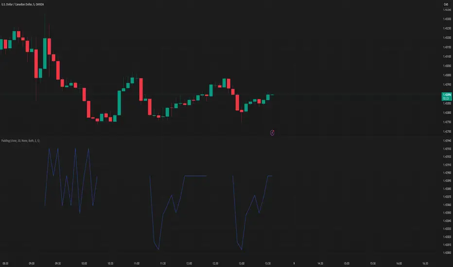
KalmanfilterLibrary "Kalmanfilter"
A sophisticated Kalman Filter implementation for financial time series analysis
@author Rocky-Studio
@version 1.0
initialize(initial_value, process_noise, measurement_noise)
Initializes Kalman Filter parameters
Parameters:
initial_value (float) : (float) The initial state estimate
process_noise (float) : (float) The process noise coefficient (Q)
measurement_noise (float) : (float) The measurement noise coefficient (R)
Returns: A tuple containing
update(prev_state, prev_covariance, measurement, process_noise, measurement_noise)
Update Kalman Filter state
Parameters:
prev_state (float)
prev_covariance (float)
measurement (float)
process_noise (float)
measurement_noise (float)
calculate_measurement_noise(price_series, length)
Adaptive measurement noise calculation
Parameters:
price_series (array)
length (int)
calculate_measurement_noise_simple(price_series)
Parameters:
price_series (array)
update_trading(prev_state, prev_velocity, prev_covariance, measurement, volatility_window)
Enhanced trading update with velocity
Parameters:
prev_state (float)
prev_velocity (float)
prev_covariance (float)
measurement (float)
volatility_window (int)
model4_update(prev_mean, prev_speed, prev_covariance, price, process_noise, measurement_noise)
Kalman Filter Model 4 implementation (Benhamou 2018)
Parameters:
prev_mean (float)
prev_speed (float)
prev_covariance (array)
price (float)
process_noise (array)
measurement_noise (float)
model4_initialize(initial_price)
Initialize Model 4 parameters
Parameters:
initial_price (float)
model4_default_process_noise()
Create default process noise matrix for Model 4
model4_calculate_measurement_noise(price_series, length)
Adaptive measurement noise calculation for Model 4
Parameters:
price_series (array)
length (int)

Two-Pole Oscillator [BigBeluga]
The Two-Pole Oscillator is an advanced smoothing oscillator designed to provide traders with precise market signals by leveraging deviation-based calculations combined with a unique two-pole filtering technique. It offers clear visual representation and actionable signals for smart trading decisions.
🔵Key Features:
Two-Pole Filtering: Smooths out the main oscillator signal to reduce noise, providing a cleaner and more reliable view of market momentum and trend strength.
// Two-pole smooth filter function
f_two_pole_filter(source, length) =>
var float smooth1 = na
var float smooth2 = na
alpha = 2.0 / (length + 1)
if na(smooth1)
smooth1 := source
else
smooth1 := (1 - alpha) * smooth1 + alpha * source
if na(smooth2)
smooth2 := smooth1
else
smooth2 := (1 - alpha) * smooth2 + alpha * smooth1
Deviation-Based Oscillator: Utilizes price deviations from the mean to generate dynamic signals, making it ideal for detecting overbought and oversold conditions.
float sma1 = ta.sma(close, 25)
float sma_n1 = ((close - sma1) - ta.sma(close - sma1, 25)) / ta.stdev(close - sma1, 25)
Signal Gradient Strength: Signals on the main oscillator line feature gradient coloring based on their proximity to the 0 level:
➔ Closer to 0: More transparent, indicating weaker signals.
➔ Closer to 1 or -1: Less transparent, highlighting stronger signals.
Level-Based Signal Validation: Parallel levels are plotted on the chart for each signal:
➔ If a level is crossed by price, the signal is invalidated, marked by an "X" at the invalidation point.
Trend Continuation
Invalidation Levels: Serve as potential stop-loss or trade-reversal zones, enabling traders to make more informed and disciplined trading decisions.
Dynamic Chart Plotting: Signals are plotted directly on the chart with corresponding levels, providing a comprehensive visual representation for easy interpretation.
🔵How It Works:
The oscillator calculates price deviation from a mean value and applies two-pole filtering to smooth the resulting signal.
Gradient-colored signals reflect their strength, with transparency indicating proximity to the 0 level on the oscillator scale.
Buy and sell signals are generated based on crossovers and crossunders of the oscillator line with a signal line.
If a level is crossed, the corresponding signal is marked with a "X" plotted on the chart at the crossover point.
🔵Use Cases:
Detecting overbought or oversold market conditions with a smoother, noise-free oscillator.
Using invalidation levels to set clear stop-loss or trade exit points.
Identifying strong momentum signals and filtering out weaker, less reliable ones.
Combining oscillator signals with price action for more precise trade entries and exits.
This indicator is perfect for traders seeking a refined approach to oscillator analysis, combining signal strength visualization with actionable invalidation levels to enhance trading precision and strategy.
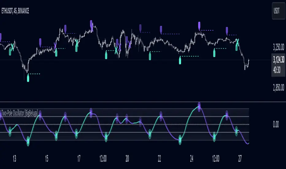
TVMC - Composite Indicator with Technical RatingsDescription:
The TVMC (Trend, Volume, Momentum, Composite) indicator is a powerful multi-component tool designed to provide traders with a comprehensive understanding of market conditions. By combining four essential technical analysis components—trend, momentum, volume, and volatility—this indicator offers clear and actionable insights to assist in decision-making.
Key Features:
1. Trend Component (TC):
* Based on MACD (Moving Average Convergence Divergence), this component analyzes the relationship between two exponential moving averages (fast and slow) to determine the prevailing market trend.
* The MACD signal is normalized to a range of -1 to +1 for consistency and clarity.
2. Momentum Component (MC):
* Utilizes RSI (Relative Strength Index) to measure the strength and speed of price movements.
* This component highlights overbought or oversold conditions, which may indicate potential market reversals.
3. Volume Confirmation (VC):
* Compares the current trading volume to its moving average over a specified period.
* High volume relative to the average confirms the validity of the current trend.
4. Volatility Filter (VF):
* Uses ATR (Average True Range) to gauge market volatility.
* Adjusts and smooths signals to reduce noise during periods of high volatility.
5. Technical Ratings Integration:
* Incorporates TradingView’s Technical Ratings, allowing users to validate signals using moving averages, oscillators, or a combination of both.
* Users can choose their preferred source of ratings for enhanced signal confirmation.
How It Works:
The TVMC indicator combines the weighted contributions of the Trend, Momentum, and Volume components, further refined by the Volatility Filter. Each component plays a specific role:
* Trend: Identifies whether the market is bullish, bearish, or neutral.
* Momentum: Highlights the strength of price action.
* Volume: Confirms whether the current price action is supported by sufficient trading activity.
* Volatility: Filters out excessive noise in volatile market conditions, providing a smoother and more reliable output.
Visualization:
1. Bullish Signals:
* The indicator line turns green and remains above the zero line, indicating upward momentum.
2. Bearish Signals:
* The indicator line turns red and falls below the zero line, signaling downward momentum.
3. Neutral Signals:
* The line is orange and stays near zero, indicating a lack of strong trend or momentum.
4. Zones:
* Horizontal lines at +30 and -30 mark strong bullish and bearish zones, respectively.
* A zero line is included for clear separation between bullish and bearish signals.
Recommended Usage:
* Best Timeframes: The indicator is optimized for higher timeframes such as 4-hour (H4) and daily (D1) charts.
* Trading Style: Suitable for swing and positional trading.
* Customization: The indicator allows users to adjust all major parameters (e.g., MACD, RSI, volume, and ATR settings) to fit their trading preferences.
Customization Options:
* Adjustable weights for Trend, Momentum, and Volume components.
* Fully configurable settings for MACD, RSI, Volume SMA, and ATR periods.
* Timeframe selection for multi-timeframe analysis.
Important Notes:
1. Originality: The TVMC indicator combines multiple analysis methods into a unique framework. It does not replicate or minimally modify existing indicators.
2. Transparency: The description is detailed enough for users to understand the methodology without requiring access to the code.
3. Clarity: The indicator is explained in a way that is accessible even to users unfamiliar with complex technical analysis tools.
Compliance with TradingView Rules:
* The indicator is written in Pine Script version 5, adhering to TradingView’s language standards.
* The description is written in English to ensure accessibility to the global community, with a clear explanation of all components and functionality.
* No promotional content, links, or unrelated references are included.
* The chart accompanying the indicator is clean and demonstrates its intended use clearly, with no additional indicators unless explicitly explained.

Ehlers Maclaurin Ultimate Smoother [CT]Ehlers Maclaurin Ultimate Smoother
Introduction
The Ehlers Maclaurin Ultimate Smoother is an innovative enhancement of the classic Ehlers SuperSmoother. By leveraging advanced Maclaurin series approximations, this indicator offers superior market analysis and signal generation.
The indicator combines Ehlers' Ultimate Smoother with Maclaurin series approximations to create a more efficient and accurate smoothing mechanism:
Input price data passes through the initial smoothing phase
Maclaurin series approximates trigonometric functions
Enhanced high-pass filter removes market noise
Final smoothing phase produces the output signal
Why the Maclaurin Approach?
The Maclaurin series is a special form of the Taylor series, centered around 0. It provides an efficient way to approximate complex functions using polynomial terms. In this indicator, we use the Maclaurin approach to improve the sine and cosine functions, resulting in:
Faster Calculations: By using polynomial approximations, we significantly reduce computational complexity.
Improved Stability: The approximation provides a more stable numerical basis for calculations.
Preservation of Precision: Despite the approximation, we maintain the precision needed for price smoothing.
Calculations
The indicator employs several key mathematical components:
Maclaurin Series Approximation:
sin(x) ≈ x - x³/3! + x⁵/5! - x⁷/7! + x⁹/9!
cos(x) ≈ 1 - x²/2! + x⁴/4! - x⁶/6! + x⁸/8!
Smoothing Algorithm:
Uses exponential smoothing with optimized coefficients
Implements high-pass filtering for noise reduction
Applies dynamic weighting based on market conditions
Mathematical Foundation
Utilizes Maclaurin series for trigonometric approximation
Implements Ehlers' smoothing principles
Incorporates advanced filtering techniques
Technical Advantages
Signal Processing:
Lag Reduction: Faster signal detection with less delay.
Noise Filtration: Effective elimination of high-frequency noise.
Precision Enhancement: Preservation of critical price movements.
Adaptive Processing: Dynamic response to market volatility.
Visual Enhancements:
Smart color intensity mapping.
Real-time visualization of trend strength.
Adaptive opacity based on movement significance.
Implementation
Core Configuration:
Plot Type: Choose between the original and the Maclaurin enhanced version.
Length: Default set to 30, optimal for daily timeframes.
hpLength: Default set to 10 for enhanced noise reduction.
Advanced Parameters:
The indicator offers advanced control with:
Dual processing modes (Original/Maclaurin).
Dynamic color intensity system.
Customizable smoothing parameters.
Professional Analysis Tools:
Accurate trend reversal identification.
Advanced support/resistance detection.
Superior performance in volatile markets.
Technical Specifications
Maclaurin Series Implementation:
The indicator employs a 5-term Maclaurin series approximation for both sine and cosine, ensuring efficient and accurate computation.
Performance Metrics
Improved processing efficiency.
Reduced memory utilization.
Increased signal accuracy.
Licensing & Attribution
© 2024 Mupsje aka CasaTropical
Professional Credits
Original Ultimate and SuperSmoother concept: John F. Ehlers
Maclaurin enhancement: Casa Tropical (CT)
www.mathsisfun.com

6 Band Parametric EQThis indicator implements a complete parametric equalizer on any data source using high-pass and low-pass filters, high and low shelving filters, and six fully configurable bell filters. Each filter stage features standard audio DSP controls including frequency, Q factor, and gain where applicable. While parametric EQ is typically used for audio processing, this implementation raises questions about the nature of filtering in technical analysis. Why stop at simple moving averages when you can shape your signal's frequency response with surgical precision? The answer may reveal more about our assumptions than our indicators.
Filter Types and Parameters
High-Pass Filter:
A high-pass filter attenuates frequency components below its cutoff frequency while passing higher frequencies. The Q parameter controls resonance at the cutoff point, with higher values creating more pronounced peaks.
Low-Pass Filter:
The low-pass filter does the opposite - it attenuates frequencies above the cutoff while passing lower frequencies. Like the high-pass, its Q parameter affects the resonance at the cutoff frequency.
High/Low Shelf Filters:
Shelf filters boost or cut all frequencies above (high shelf) or below (low shelf) the target frequency. The slope parameter determines the steepness of the transition around the target frequency , with a value of 1.0 creating a gentle slope and lower values making the transition more abrupt. The gain parameter sets the amount of boost or cut in decibels.
Bell Filters:
Bell (or peaking) filters create a boost or cut centered around a specific frequency. A bell filter's frequency parameter determines the center point of the effect, while Q controls the width of the affected frequency range - higher Q values create a narrower bandwidth. The gain parameter defines the amount of boost or cut in decibels.
All filters run in series, processing the signal in this order: high-pass → low shelf → bell filters → high shelf → low-pass. Each stage can be independently enabled or bypassed.
The frequency parameter for all filters represents the period length of the targeted frequency component. Lower values target higher frequencies and vice versa. All gain values are in decibels, where positive values boost and negative values cut.
The 6-Band Parametric EQ combines these filters into a comprehensive frequency shaping tool. Just as audio engineers use parametric EQs to sculpt sound, this indicator lets you shape market data's frequency components with surgical precision. But beyond its technical implementation, this indicator serves as a thought experiment about the nature of filtering in technical analysis. While traditional indicators often rely on simple moving averages or single-frequency filters, the parametric EQ takes this concept to its logical extreme - offering complete control over the frequency domain of price action. Whether this level of filtering precision is useful for analysis is perhaps less important than what it reveals about our assumptions regarding market data and its frequency components.
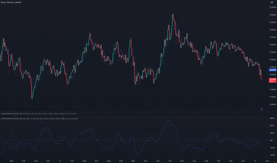
Wave Smoother [WS]The Wave Smoother is a unique FIR filter built from the interaction of two trigonometric waves. A cosine carrier wave is modulated by a sine wave at half the carrier's period, creating smooth transitions and controlled undershoot. The Phase parameter (0° to 119°) adjusts the modulating wave's phase, affecting both response time and undershoot characteristics. At 30° phase the impulse response starts at 0.5 and exhibits gentle undershoot, providing balanced smoothing. Higher phase values reduce ramp-up time and increase undershoot - this undershoot in the impulse response creates overshooting behavior in the filter's output, which helps reduce lag and speed up the response. The default 70° phase setting provides maximum speed while maintaining stability, though practical settings can range from 30° to 70°. The filter's impulse response consists entirely of smooth curves, ensuring consistent behavior across all settings. This design offers traders flexible control over the smoothing-speed trade-off while maintaining reliable signal generation.
