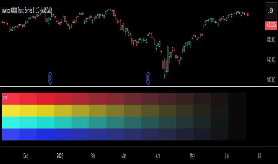
Color█ OVERVIEW
This library is a Pine Script® programming tool for advanced color processing. It provides a comprehensive set of functions for specifying and analyzing colors in various color spaces, mixing and manipulating colors, calculating custom gradients and schemes, detecting contrast, and converting colors to or from hexadecimal strings.
█ CONCEPTS
Color
Color refers to how we interpret light of different wavelengths in the visible spectrum . The colors we see from an object represent the light wavelengths that it reflects, emits, or transmits toward our eyes. Some colors, such as blue and red, correspond directly to parts of the spectrum. Others, such as magenta, arise from a combination of wavelengths to which our minds assign a single color.
The human interpretation of color lends itself to many uses in our world. In the context of financial data analysis, the effective use of color helps transform raw data into insights that users can understand at a glance. For example, colors can categorize series, signal market conditions and sessions, and emphasize patterns or relationships in data.
Color models and spaces
A color model is a general mathematical framework that describes colors using sets of numbers. A color space is an implementation of a specific color model that defines an exact range (gamut) of reproducible colors based on a set of primary colors , a reference white point , and sometimes additional parameters such as viewing conditions.
There are numerous different color spaces — each describing the characteristics of color in unique ways. Different spaces carry different advantages, depending on the application. Below, we provide a brief overview of the concepts underlying the color spaces supported by this library.
RGB
RGB is one of the most well-known color models. It represents color as an additive mixture of three primary colors — red, green, and blue lights — with various intensities. Each cone cell in the human eye responds more strongly to one of the three primaries, and the average person interprets the combination of these lights as a distinct color (e.g., pure red + pure green = yellow).
The sRGB color space is the most common RGB implementation. Developed by HP and Microsoft in the 1990s, sRGB provided a standardized baseline for representing color across CRT monitors of the era, which produced brightness levels that did not increase linearly with the input signal. To match displays and optimize brightness encoding for human sensitivity, sRGB applied a nonlinear transformation to linear RGB signals, often referred to as gamma correction . The result produced more visually pleasing outputs while maintaining a simple encoding. As such, sRGB quickly became a standard for digital color representation across devices and the web. To this day, it remains the default color space for most web-based content.
TradingView charts and Pine Script `color.*` built-ins process color data in sRGB. The red, green, and blue channels range from 0 to 255, where 0 represents no intensity, and 255 represents maximum intensity. Each combination of red, green, and blue values represents a distinct color, resulting in a total of 16,777,216 displayable colors.
CIE XYZ and xyY
The XYZ color space, developed by the International Commission on Illumination (CIE) in 1931, aims to describe all color sensations that a typical human can perceive. It is a cornerstone of color science, forming the basis for many color spaces used today. XYZ, and the derived xyY space, provide a universal representation of color that is not tethered to a particular display. Many widely used color spaces, including sRGB, are defined relative to XYZ or derived from it.
The CIE built the color space based on a series of experiments in which people matched colors they perceived from mixtures of lights. From these experiments, the CIE developed color-matching functions to calculate three components — X, Y, and Z — which together aim to describe a standard observer's response to visible light. X represents a weighted response to light across the color spectrum, with the highest contribution from long wavelengths (e.g., red). Y represents a weighted response to medium wavelengths (e.g., green), and it corresponds to a color's relative luminance (i.e., brightness). Z represents a weighted response to short wavelengths (e.g., blue).
From the XYZ space, the CIE developed the xyY chromaticity space, which separates a color's chromaticity (hue and colorfulness) from luminance. The CIE used this space to define the CIE 1931 chromaticity diagram , which represents the full range of visible colors at a given luminance. In color science and lighting design, xyY is a common means for specifying colors and visualizing the supported ranges of other color spaces.
CIELAB and Oklab
The CIELAB (L*a*b*) color space, derived from XYZ by the CIE in 1976, expresses colors based on opponent process theory. The L* component represents perceived lightness, and the a* and b* components represent the balance between opposing unique colors. The a* value specifies the balance between green and red , and the b* value specifies the balance between blue and yellow .
The primary intention of CIELAB was to provide a perceptually uniform color space, where fixed-size steps through the space correspond to uniform perceived changes in color. Although relatively uniform, the color space has been found to exhibit some non-uniformities, particularly in the blue part of the color spectrum. Regardless, modern applications often use CIELAB to estimate perceived color differences and calculate smooth color gradients.
In 2020, a new LAB-oriented color space, Oklab , was introduced by Björn Ottosson as an attempt to rectify the non-uniformities of other perceptual color spaces. Similar to CIELAB, the L value in Oklab represents perceived lightness, and the a and b values represent the balance between opposing unique colors. Oklab has gained widespread adoption as a perceptual space for color processing, with support in the latest CSS Color specifications and many software applications.
Cylindrical models
A cylindrical-coordinate model transforms an underlying color model, such as RGB or LAB, into an alternative expression of color information that is often more intuitive for the average person to use and understand.
Instead of a mixture of primary colors or opponent pairs, these models represent color as a hue angle on a color wheel , with additional parameters that describe other qualities such as lightness and colorfulness (a general term for concepts like chroma and saturation). In cylindrical-coordinate spaces, users can select a color and modify its lightness or other qualities without altering the hue.
The three most common RGB-based models are HSL (Hue, Saturation, Lightness), HSV (Hue, Saturation, Value), and HWB (Hue, Whiteness, Blackness). All three define hue angles in the same way, but they define colorfulness and lightness differently. Although they are not perceptually uniform, HSL and HSV are commonplace in color pickers and gradients.
For CIELAB and Oklab, the cylindrical-coordinate versions are CIELCh and Oklch , which express color in terms of perceived lightness, chroma, and hue. They offer perceptually uniform alternatives to RGB-based models. These spaces create unique color wheels, and they have more strict definitions of lightness and colorfulness. Oklch is particularly well-suited for generating smooth, perceptual color gradients.
Alpha and transparency
Many color encoding schemes include an alpha channel, representing opacity . Alpha does not help define a color in a color space; it determines how a color interacts with other colors in the display. Opaque colors appear with full intensity on the screen, whereas translucent (semi-opaque) colors blend into the background. Colors with zero opacity are invisible.
In Pine Script, there are two ways to specify a color's alpha:
• Using the `transp` parameter of the built-in `color.*()` functions. The specified value represents transparency (the opposite of opacity), which the functions translate into an alpha value.
• Using eight-digit hexadecimal color codes. The last two digits in the code represent alpha directly.
A process called alpha compositing simulates translucent colors in a display. It creates a single displayed color by mixing the RGB channels of two colors (foreground and background) based on alpha values, giving the illusion of a semi-opaque color placed over another color. For example, a red color with 80% transparency on a black background produces a dark shade of red.
Hexadecimal color codes
A hexadecimal color code (hex code) is a compact representation of an RGB color. It encodes a color's red, green, and blue values into a sequence of hexadecimal ( base-16 ) digits. The digits are numerals ranging from `0` to `9` or letters from `a` (for 10) to `f` (for 15). Each set of two digits represents an RGB channel ranging from `00` (for 0) to `ff` (for 255).
Pine scripts can natively define colors using hex codes in the format `#rrggbbaa`. The first set of two digits represents red, the second represents green, and the third represents blue. The fourth set represents alpha . If unspecified, the value is `ff` (fully opaque). For example, `#ff8b00` and `#ff8b00ff` represent an opaque orange color. The code `#ff8b0033` represents the same color with 80% transparency.
Gradients
A color gradient maps colors to numbers over a given range. Most color gradients represent a continuous path in a specific color space, where each number corresponds to a mix between a starting color and a stopping color. In Pine, coders often use gradients to visualize value intensities in plots and heatmaps, or to add visual depth to fills.
The behavior of a color gradient depends on the mixing method and the chosen color space. Gradients in sRGB usually mix along a straight line between the red, green, and blue coordinates of two colors. In cylindrical spaces such as HSL, a gradient often rotates the hue angle through the color wheel, resulting in more pronounced color transitions.
Color schemes
A color scheme refers to a set of colors for use in aesthetic or functional design. A color scheme usually consists of just a few distinct colors. However, depending on the purpose, a scheme can include many colors.
A user might choose palettes for a color scheme arbitrarily, or generate them algorithmically. There are many techniques for calculating color schemes. A few simple, practical methods are:
• Sampling a set of distinct colors from a color gradient.
• Generating monochromatic variants of a color (i.e., tints, tones, or shades with matching hues).
• Computing color harmonies — such as complements, analogous colors, triads, and tetrads — from a base color.
This library includes functions for all three of these techniques. See below for details.
█ CALCULATIONS AND USE
Hex string conversion
The `getHexString()` function returns a string containing the eight-digit hexadecimal code corresponding to a "color" value or set of sRGB and transparency values. For example, `getHexString(255, 0, 0)` returns the string `"#ff0000ff"`, and `getHexString(color.new(color.red, 80))` returns `"#f2364533"`.
The `hexStringToColor()` function returns the "color" value represented by a string containing a six- or eight-digit hex code. The `hexStringToRGB()` function returns a tuple containing the sRGB and transparency values. For example, `hexStringToColor("#f23645")` returns the same value as color.red .
Programmers can use these functions to parse colors from "string" inputs, perform string-based color calculations, and inspect color data in text outputs such as Pine Logs and tables.
Color space conversion
All other `get*()` functions convert a "color" value or set of sRGB channels into coordinates in a specific color space, with transparency information included. For example, the tuple returned by `getHSL()` includes the color's hue, saturation, lightness, and transparency values.
To convert data from a color space back to colors or sRGB and transparency values, use the corresponding `*toColor()` or `*toRGB()` functions for that space (e.g., `hslToColor()` and `hslToRGB()`).
Programmers can use these conversion functions to process inputs that define colors in different ways, perform advanced color manipulation, design custom gradients, and more.
The color spaces this library supports are:
• sRGB
• Linear RGB (RGB without gamma correction)
• HSL, HSV, and HWB
• CIE XYZ and xyY
• CIELAB and CIELCh
• Oklab and Oklch
Contrast-based calculations
Contrast refers to the difference in luminance or color that makes one color visible against another. This library features two functions for calculating luminance-based contrast and detecting themes.
The `contrastRatio()` function calculates the contrast between two "color" values based on their relative luminance (the Y value from CIE XYZ) using the formula from version 2 of the Web Content Accessibility Guidelines (WCAG) . This function is useful for identifying colors that provide a sufficient brightness difference for legibility.
The `isLightTheme()` function determines whether a specified background color represents a light theme based on its contrast with black and white. Programmers can use this function to define conditional logic that responds differently to light and dark themes.
Color manipulation and harmonies
The `negative()` function calculates the negative (i.e., inverse) of a color by reversing the color's coordinates in either the sRGB or linear RGB color space. This function is useful for calculating high-contrast colors.
The `grayscale()` function calculates a grayscale form of a specified color with the same relative luminance.
The functions `complement()`, `splitComplements()`, `analogousColors()`, `triadicColors()`, `tetradicColors()`, `pentadicColors()`, and `hexadicColors()` calculate color harmonies from a specified source color within a given color space (HSL, CIELCh, or Oklch). The returned harmonious colors represent specific hue rotations around a color wheel formed by the chosen space, with the same defined lightness, saturation or chroma, and transparency.
Color mixing and gradient creation
The `add()` function simulates combining lights of two different colors by additively mixing their linear red, green, and blue components, ignoring transparency by default. Users can calculate a transparency-weighted mixture by setting the `transpWeight` argument to `true`.
The `overlay()` function estimates the color displayed on a TradingView chart when a specific foreground color is over a background color. This function aids in simulating stacked colors and analyzing the effects of transparency.
The `fromGradient()` and `fromMultiStepGradient()` functions calculate colors from gradients in any of the supported color spaces, providing flexible alternatives to the RGB-based color.from_gradient() function. The `fromGradient()` function calculates a color from a single gradient. The `fromMultiStepGradient()` function calculates a color from a piecewise gradient with multiple defined steps. Gradients are useful for heatmaps and for coloring plots or drawings based on value intensities.
Scheme creation
Three functions in this library calculate palettes for custom color schemes. Scripts can use these functions to create responsive color schemes that adjust to calculated values and user inputs.
The `gradientPalette()` function creates an array of colors by sampling a specified number of colors along a gradient from a base color to a target color, in fixed-size steps.
The `monoPalette()` function creates an array containing monochromatic variants (tints, tones, or shades) of a specified base color. Whether the function mixes the color toward white (for tints), a form of gray (for tones), or black (for shades) depends on the `grayLuminance` value. If unspecified, the function automatically chooses the mix behavior with the highest contrast.
The `harmonyPalette()` function creates a matrix of colors. The first column contains the base color and specified harmonies, e.g., triadic colors. The columns that follow contain tints, tones, or shades of the harmonic colors for additional color choices, similar to `monoPalette()`.
█ EXAMPLE CODE
The example code at the end of the script generates and visualizes color schemes by processing user inputs. The code builds the scheme's palette based on the "Base color" input and the additional inputs in the "Settings/Inputs" tab:
• "Palette type" specifies whether the palette uses a custom gradient, monochromatic base color variants, or color harmonies with monochromatic variants.
• "Target color" sets the top color for the "Gradient" palette type.
• The "Gray luminance" inputs determine variation behavior for "Monochromatic" and "Harmony" palette types. If "Auto" is selected, the palette mixes the base color toward white or black based on its brightness. Otherwise, it mixes the color toward the grayscale color with the specified relative luminance (from 0 to 1).
• "Harmony type" specifies the color harmony used in the palette. Each row in the palette corresponds to one of the harmonious colors, starting with the base color.
The code creates a table on the first bar to display the collection of calculated colors. Each cell in the table shows the color's `getHexString()` value in a tooltip for simple inspection.
Look first. Then leap.
█ EXPORTED FUNCTIONS
Below is a complete list of the functions and overloads exported by this library.
getRGB(source)
Retrieves the sRGB red, green, blue, and transparency components of a "color" value.
getHexString(r, g, b, t)
(Overload 1 of 2) Converts a set of sRGB channel values to a string representing the corresponding color's hexadecimal form.
getHexString(source)
(Overload 2 of 2) Converts a "color" value to a string representing the sRGB color's hexadecimal form.
hexStringToRGB(source)
Converts a string representing an sRGB color's hexadecimal form to a set of decimal channel values.
hexStringToColor(source)
Converts a string representing an sRGB color's hexadecimal form to a "color" value.
getLRGB(r, g, b, t)
(Overload 1 of 2) Converts a set of sRGB channel values to a set of linear RGB values with specified transparency information.
getLRGB(source)
(Overload 2 of 2) Retrieves linear RGB channel values and transparency information from a "color" value.
lrgbToRGB(lr, lg, lb, t)
Converts a set of linear RGB channel values to a set of sRGB values with specified transparency information.
lrgbToColor(lr, lg, lb, t)
Converts a set of linear RGB channel values and transparency information to a "color" value.
getHSL(r, g, b, t)
(Overload 1 of 2) Converts a set of sRGB channels to a set of HSL values with specified transparency information.
getHSL(source)
(Overload 2 of 2) Retrieves HSL channel values and transparency information from a "color" value.
hslToRGB(h, s, l, t)
Converts a set of HSL channel values to a set of sRGB values with specified transparency information.
hslToColor(h, s, l, t)
Converts a set of HSL channel values and transparency information to a "color" value.
getHSV(r, g, b, t)
(Overload 1 of 2) Converts a set of sRGB channels to a set of HSV values with specified transparency information.
getHSV(source)
(Overload 2 of 2) Retrieves HSV channel values and transparency information from a "color" value.
hsvToRGB(h, s, v, t)
Converts a set of HSV channel values to a set of sRGB values with specified transparency information.
hsvToColor(h, s, v, t)
Converts a set of HSV channel values and transparency information to a "color" value.
getHWB(r, g, b, t)
(Overload 1 of 2) Converts a set of sRGB channels to a set of HWB values with specified transparency information.
getHWB(source)
(Overload 2 of 2) Retrieves HWB channel values and transparency information from a "color" value.
hwbToRGB(h, w, b, t)
Converts a set of HWB channel values to a set of sRGB values with specified transparency information.
hwbToColor(h, w, b, t)
Converts a set of HWB channel values and transparency information to a "color" value.
getXYZ(r, g, b, t)
(Overload 1 of 2) Converts a set of sRGB channels to a set of XYZ values with specified transparency information.
getXYZ(source)
(Overload 2 of 2) Retrieves XYZ channel values and transparency information from a "color" value.
xyzToRGB(x, y, z, t)
Converts a set of XYZ channel values to a set of sRGB values with specified transparency information
xyzToColor(x, y, z, t)
Converts a set of XYZ channel values and transparency information to a "color" value.
getXYY(r, g, b, t)
(Overload 1 of 2) Converts a set of sRGB channels to a set of xyY values with specified transparency information.
getXYY(source)
(Overload 2 of 2) Retrieves xyY channel values and transparency information from a "color" value.
xyyToRGB(xc, yc, y, t)
Converts a set of xyY channel values to a set of sRGB values with specified transparency information.
xyyToColor(xc, yc, y, t)
Converts a set of xyY channel values and transparency information to a "color" value.
getLAB(r, g, b, t)
(Overload 1 of 2) Converts a set of sRGB channels to a set of CIELAB values with specified transparency information.
getLAB(source)
(Overload 2 of 2) Retrieves CIELAB channel values and transparency information from a "color" value.
labToRGB(l, a, b, t)
Converts a set of CIELAB channel values to a set of sRGB values with specified transparency information.
labToColor(l, a, b, t)
Converts a set of CIELAB channel values and transparency information to a "color" value.
getOKLAB(r, g, b, t)
(Overload 1 of 2) Converts a set of sRGB channels to a set of Oklab values with specified transparency information.
getOKLAB(source)
(Overload 2 of 2) Retrieves Oklab channel values and transparency information from a "color" value.
oklabToRGB(l, a, b, t)
Converts a set of Oklab channel values to a set of sRGB values with specified transparency information.
oklabToColor(l, a, b, t)
Converts a set of Oklab channel values and transparency information to a "color" value.
getLCH(r, g, b, t)
(Overload 1 of 2) Converts a set of sRGB channels to a set of CIELCh values with specified transparency information.
getLCH(source)
(Overload 2 of 2) Retrieves CIELCh channel values and transparency information from a "color" value.
lchToRGB(l, c, h, t)
Converts a set of CIELCh channel values to a set of sRGB values with specified transparency information.
lchToColor(l, c, h, t)
Converts a set of CIELCh channel values and transparency information to a "color" value.
getOKLCH(r, g, b, t)
(Overload 1 of 2) Converts a set of sRGB channels to a set of Oklch values with specified transparency information.
getOKLCH(source)
(Overload 2 of 2) Retrieves Oklch channel values and transparency information from a "color" value.
oklchToRGB(l, c, h, t)
Converts a set of Oklch channel values to a set of sRGB values with specified transparency information.
oklchToColor(l, c, h, t)
Converts a set of Oklch channel values and transparency information to a "color" value.
contrastRatio(value1, value2)
Calculates the contrast ratio between two colors values based on the formula from version 2 of the Web Content Accessibility Guidelines (WCAG).
isLightTheme(source)
Detects whether a background color represents a light theme or dark theme, based on the amount of contrast between the color and the white and black points.
grayscale(source)
Calculates the grayscale version of a color with the same relative luminance (i.e., brightness).
negative(source, colorSpace)
Calculates the negative (i.e., inverted) form of a specified color.
complement(source, colorSpace)
Calculates the complementary color for a `source` color using a cylindrical color space.
analogousColors(source, colorSpace)
Calculates the analogous colors for a `source` color using a cylindrical color space.
splitComplements(source, colorSpace)
Calculates the split-complementary colors for a `source` color using a cylindrical color space.
triadicColors(source, colorSpace)
Calculates the two triadic colors for a `source` color using a cylindrical color space.
tetradicColors(source, colorSpace, square)
Calculates the three square or rectangular tetradic colors for a `source` color using a cylindrical color space.
pentadicColors(source, colorSpace)
Calculates the four pentadic colors for a `source` color using a cylindrical color space.
hexadicColors(source, colorSpace)
Calculates the five hexadic colors for a `source` color using a cylindrical color space.
add(value1, value2, transpWeight)
Additively mixes two "color" values, with optional transparency weighting.
overlay(fg, bg)
Estimates the resulting color that appears on the chart when placing one color over another.
fromGradient(value, bottomValue, topValue, bottomColor, topColor, colorSpace)
Calculates the gradient color that corresponds to a specific value based on a defined value range and color space.
fromMultiStepGradient(value, steps, colors, colorSpace)
Calculates a multi-step gradient color that corresponds to a specific value based on an array of step points, an array of corresponding colors, and a color space.
gradientPalette(baseColor, stopColor, steps, strength, model)
Generates a palette from a gradient between two base colors.
monoPalette(baseColor, grayLuminance, variations, strength, colorSpace)
Generates a monochromatic palette from a specified base color.
harmonyPalette(baseColor, harmonyType, grayLuminance, variations, strength, colorSpace)
Generates a palette consisting of harmonious base colors and their monochromatic variants.
Gradient
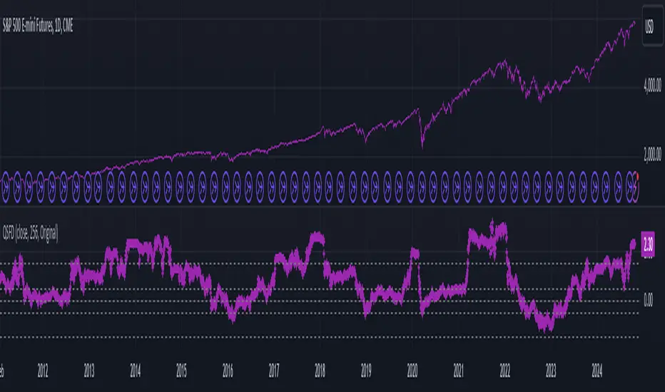
Quick scan for drift🙏🏻
ML based algorading is all about detecting any kind of non-randomness & exploiting it, kinda speculative stuff, not my way, but still...
Drift is one of the patterns that can be exploited, because pure random walks & noise aint got no drift.
This is an efficient method to quickly scan tons of timeseries on the go & detect the ones with drift by simply checking wherther drift < -0.5 or drift > 0.5. The code can be further optimized both in general and for specific needs, but I left it like dat for clarity so you can understand how it works in a minute not in an hour
^^ proving 0.5 and -0.5 are natural limits with no need to optimize anything, we simply put the metric on random noise and see it sits in between -0.5 and 0.5
You can simply take this one and never check anything again if you require numerous live scans on the go. The metric is purely geometrical, no connection to stats, TSA, DSA or whatever. I've tested numerous formulas involving other scaling techniques, drift estimates etc (even made a recursive algo that had a great potential to be written about in a paper, but not this time I gues lol), this one has the highest info gain aka info content.
The timeseries filtered by this lil metric can be further analyzed & modelled with more sophisticated tools.
Live Long and Prosper
P.S.: there's no such thing as polynomial trend/drift, it's alwasy linear, these curves you see are just really long cycles
P.S.: does cheer still work on TV? @admin
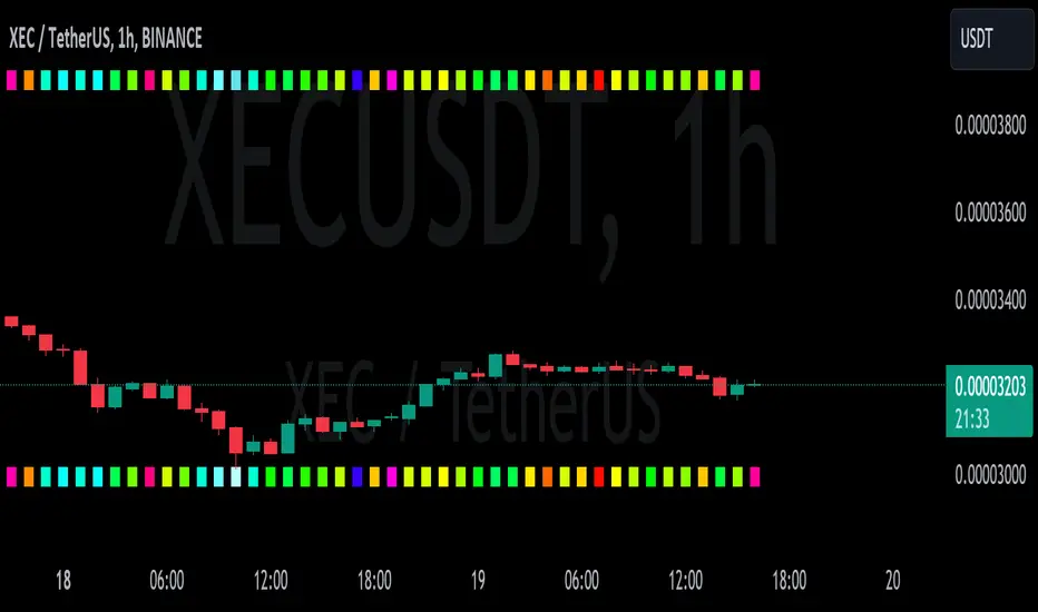
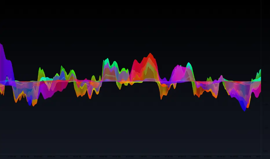
Gradient Value Overlay
This script helps with identifying certain conditions without cluttering too much of the candles.
Some use cases:
It helps identify rsi low and high values.
Directional price movement becoming difficult.
low and high volume.
it uses a percent rank to distinguish low and high values.
It then uses a gradient to match the percentile rank to heatmap type colors.
i.e. dark blue for lowest volume, white for highest volume.
Current options are:
max bars to use.
approximate color - This value will attempt to give an approximation of what the color might be for the candle close.
e.g. If you're on the 1-hour chart, and only 30 minutes have past, it will multiple the current volume by 1.5. As time passes, if no volume comes in eventually, it will multiply current volume by 1.
This approximate value is only set to work with volume-based options.
option - select the type of value you'd like to see the gradient for.
timeframe - get values from a different chart timeframe.
on/off - turns the gradient on or off.
Gradient type - color wheel or heatmap. Currently these are the only two gardient options.
color wheel's colors for low to high values:
color wheel's current colors:
dark blue
purple
pink
red
orange
yellow
green
teal
white
heatmap's current colors from low values to high values:
dark blue
purple
pink
red
orange
yellow
white
reverse gradient - will reverse the colors so dark blue will be the high value and white will be the low value. Some charts based on previous data; you might need to switch the gradient colors.
moving average length while inside timeframe - an exponential moving average is applied to the values. At 1, there is no moving average applied.
Use case for this is to smooth out the gradient.
An example use case - if your currently on the 1-hour chart, you can set the timeframe to 1 minute and then the moving average length inside timeframe to 60. You will then be seeing the color sixty 1-minute bars.
current timeframe moving average length - an exponential moving average applied to current gradient (helps with smoothing gradient).
Smooth, further smooths values.
There is no set rule for what moving average lengths to use. Adjust timeframe, and moving average lengths to get an insight.
Keltner Channels Bands (RMA)Keltner Channel Bands
These normally consist of:
Keltner Channel Upper Band = EMA + Multiplier ∗ ATR
Keltner Channel Lower Band = EMA − Multiplier ∗ ATR
However instead of using ATR we are using RMA
This gives us a much smoother take of the KCB
We are also using 2 sets of bands built on 1 Moving average, this is a common set up for mean reversion strategies.
This can often be paired with RSI for lower timeframe divergences
Divergence
This is using the RSI to calculate when price sets new lows/highs whilst the RSI movement is in the opposite direction.
The way this is calculated is slightly different to traditional divergence scripts. instead of looking for pivot highs/lows in the RSI we are logging the RSI value when price makes it pivot highs/lows.
Gradient Bands
The Gradient Colouring on the bands is measuring how long price has been either side of the MA.
As Keltner bands are commonly used as a mean reversion strategy, I thought it would be useful to see how long price has been trending in a certain direction, the stronger the colours get,
the longer price has been trending that direction which could suggest we are looking for a retrace soon.
Alerts
Alerts included let you choose whether you want to receive an alert for the inside, outside or both band touches.
To set up these alerts, simply toggle them on in the settings, then click on the 3 dots next to the indicators name, from there you click 'Add Alert'.
From there you can customise the alert settings but make sure to leave the 2 top boxes which control the alert conditions. They will be default selected onto your correct settings, the rest you may want to change.
Once you create the alert, it will then trigger as soon as price touches your chosen inside/outside band.
Suggestions
Please feel free to offer any suggestions which you think could improve the script
Disclaimer
The default settings/parameters were shared by Jimtalbott, feel free to play about with the and use this code to make your own strategies.

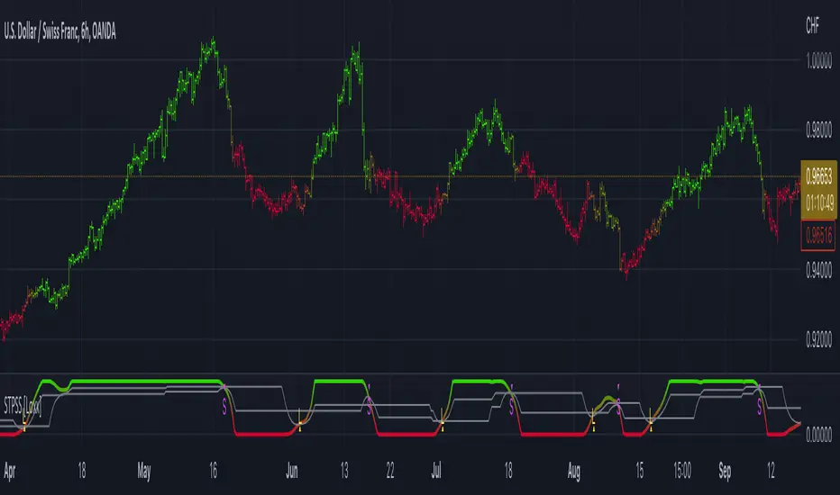
Stochastic of Two-Pole SuperSmoother [Loxx]Stochastic of Two-Pole SuperSmoother is a Stochastic Indicator that takes as input Two-Pole SuperSmoother of price. Includes gradient coloring and Discontinued Signal Lines signals with alerts.
What is Ehlers ; Two-Pole Super Smoother?
From "Cycle Analytics for Traders Advanced Technical Trading Concepts" by John F. Ehlers
A SuperSmoother filter is used anytime a moving average of any type would otherwise be used, with the result that the SuperSmoother filter output would have substantially less lag for an equivalent amount of smoothing produced by the moving average. For example, a five-bar SMA has a cutoff period of approximately 10 bars and has two bars of lag. A SuperSmoother filter with a cutoff period of 10 bars has a lag a half bar larger than the two-pole modified Butterworth filter.Therefore, such a SuperSmoother filter has a maximum lag of approximately 1.5 bars and even less lag into the attenuation band of the filter. The differential in lag between moving average and SuperSmoother filter outputs becomes even larger when the cutoff periods are larger.
Market data contain noise, and removal of noise is the reason for using smoothing filters. In fact, market data contain several kinds of noise. I’ll group one kind of noise as systemic, caused by the random events of trades being exercised. A second kind of noise is aliasing noise, caused by the use of sampled data. Aliasing noise is the dominant term in the data for shorter cycle periods.
It is easy to think of market data as being a continuous waveform, but it is not. Using the closing price as representative for that bar constitutes one sample point. It doesn’t matter if you are using an average of the high and low instead of the close, you are still getting one sample per bar. Since sampled data is being used, there are some dSP aspects that must be considered. For example, the shortest analysis period that is possible (without aliasing)2 is a two-bar cycle.This is called the Nyquist frequency, 0.5 cycles per sample.A perfect two-bar sine wave cycle sampled at the peaks becomes a square wave due to sampling. However, sampling at the cycle peaks can- not be guaranteed, and the interference between the sampling frequency and the data frequency creates the aliasing noise.The noise is reduced as the data period is longer. For example, a four-bar cycle means there are four samples per cycle. Because there are more samples, the sampled data are a better replica of the sine wave component. The replica is better yet for an eight-bar data component.The improved fidelity of the sampled data means the aliasing noise is reduced at longer and longer cycle periods.The rate of reduction is 6 dB per octave. My experience is that the systemic noise rarely is more than 10 dB below the level of cyclic information, so that we create two conditions for effective smoothing of aliasing noise:
1. It is difficult to use cycle periods shorter that two octaves below the Nyquist frequency.That is, an eight-bar cycle component has a quantization noise level 12 dB below the noise level at the Nyquist frequency. longer cycle components therefore have a systemic noise level that exceeds the aliasing noise level.
2. A smoothing filter should have sufficient selectivity to reduce aliasing noise below the systemic noise level. Since aliasing noise increases at the rate of 6 dB per octave above a selected filter cutoff frequency and since the SuperSmoother attenuation rate is 12 dB per octave, the Super- Smoother filter is an effective tool to virtually eliminate aliasing noise in the output signal.
What are DSL Discontinued Signal Line?
A lot of indicators are using signal lines in order to determine the trend (or some desired state of the indicator) easier. The idea of the signal line is easy : comparing the value to it's smoothed (slightly lagging) state, the idea of current momentum/state is made.
Discontinued signal line is inheriting that simple signal line idea and it is extending it : instead of having one signal line, more lines depending on the current value of the indicator.
"Signal" line is calculated the following way :
When a certain level is crossed into the desired direction, the EMA of that value is calculated for the desired signal line
When that level is crossed into the opposite direction, the previous "signal" line value is simply "inherited" and it becomes a kind of a level
This way it becomes a combination of signal lines and levels that are trying to combine both the good from both methods.
In simple terms, DSL uses the concept of a signal line and betters it by inheriting the previous signal line's value & makes it a level.
Included:
Bar coloring
Alerts
Signals
Loxx's Expanded Source Types
FDI-Adaptive Non-Lag Moving Average [Loxx]FDI-Adaptive Non-Lag Moving Average is a Fractal Dimension Index adaptive Non-Lag moving Average. This acts more like a trend coloring indictor with gradient coloring.
What is the Fractal Dimension Index?
The goal of the fractal dimension index is to determine whether the market is trending or in a trading range. It does not measure the direction of the trend. A value less than 1.5 indicates that the price series is persistent or that the market is trending. Lower values of the FDI indicate a stronger trend. A value greater than 1.5 indicates that the market is in a trading range and is acting in a more random fashion.
Included
Bar coloring
Loxx's Expanded Source Types

HSV and HSL gradient Tools ( Built-in Drop-in replacement )Library "hsvColor"
HSV and HSL Gradient Tool Alternatives and helpers. Demo'd is built-in in the middle with HSL/HSV gradients on top/bottom
TODO: Solve for #000000 issue
rgbhsv(_col)
RGB Color to HSV Values
Parameters:
_col : Color input (#abc012 or color.name or color.rgb(0,0,0,0))
Returns: values
rgbhsv(_r, _g, _b, _t)
RGB Color to HSV Values
Parameters:
_r : Red 0 - 255
_g : Green 0 - 255
_b : Blue 0 - 255
_t : Transp 0 - 100
Returns: values
hsv(_h, _s, _v, _a)
HSV colors, Auto fix if past boundaries
Parameters:
_h : Hue Input (-360 - 360) or further
_s : Saturation 0.- 1.
_v : Value 0.- 1.
_a : Alpha 0.- 1.
Returns: Color output
hue(_col)
returns 0-359 hue on color wheel
Parameters:
_col :
Returns: 360 degree hue value
hsv_gradient(signal, _startVal, _endVal, _startCol, _endCol)
Color Gradient Replacement Function for HSV calculated Gradents
Parameters:
signal : Control signal
_startVal : start color limit
_endVal : end color limit
_startCol : start color
_endCol : end color
Returns: HSV calculated gradient
hsl_gradient(signal, _startVal, _endVal, _startCol, _endCol)
Color Gradient Replacement Function for HSV calculated Gradents
Parameters:
signal : Control signal
_startVal : start color limit
_endVal : end color limit
_startCol : start color
_endCol : end color
Returns: HSV calculated gradient
RSI - colour fillThis script showcases the new (overload) feature regarding the fill() function! 🥳
2 plots could be filled before, but with just 1 colour per bar, now the colour can be a gradient type.
In this example we have 2 plots
- rsiPlot , which plots the rsi value
- centerPlot, which plots the value 50 ('centre line')
Explanation of colour fill in the zone 50-80
Default when rsi > 50
- a bottom value is set at 50 (associated with colour aqua)
- and a top value is set at 80 (associated with colour red)
This zone (bottom -> top value) is filled with a gradient colour (50 - aqua -> 80 - red)
When rsi is towards 80, you see a red coloured zone at the rsi value,
while when rsi is around 50, you'll only see the colour aqua
The same principle is applied in the zone 20-50 when rsi < 50
Cheers!
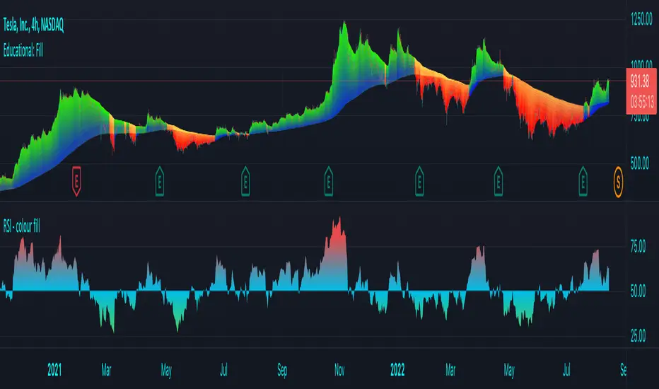
Educational: FillThis script showcases the latest feature of colour fill between lines with gradient
There are 17 ema's, all with adjustable lengths.
In the settings there are 3 options: '1' , '2' , and '1 & 2' :
Option '1'
Here the highest - lowest lines are filled with a gradient colour,
dependable where the 3rd highest/lowest ema is situated in regard of these 2 lines:
Option '2'
Here the colour fill is applied between every ema and the one next to it.
The gradient colour is dependable where the ema is situated in regard of the highest - lowest line:
Option '1 & 2'
A combination of both options:
The setting 'switch colours at ema x' regulates the switch between bullish and bearish colours.
When close is above the chosen ema -> bullish colours, when below -> bearish colours.
Examples of other settings of 'switch colours at ema x' :
Colour switch when close above/below:
ema 14
ema 11
ema 8
ema 5
ema 2
The colours can be set below, both for option '1' and '2'
Cheers!

T3 Velocity [Loxx]T3 Velocity is a simple velocity indicator using T3 moving average that uses gradient colors to better identify trends.
What is the T3 moving average?
Better Moving Averages Tim Tillson
November 1, 1998
Tim Tillson is a software project manager at Hewlett-Packard, with degrees in Mathematics and Computer Science. He has privately traded options and equities for 15 years.
Introduction
"Digital filtering includes the process of smoothing, predicting, differentiating, integrating, separation of signals, and removal of noise from a signal. Thus many people who do such things are actually using digital filters without realizing that they are; being unacquainted with the theory, they neither understand what they have done nor the possibilities of what they might have done."
This quote from R. W. Hamming applies to the vast majority of indicators in technical analysis . Moving averages, be they simple, weighted, or exponential, are lowpass filters; low frequency components in the signal pass through with little attenuation, while high frequencies are severely reduced.
"Oscillator" type indicators (such as MACD , Momentum, Relative Strength Index ) are another type of digital filter called a differentiator.
Tushar Chande has observed that many popular oscillators are highly correlated, which is sensible because they are trying to measure the rate of change of the underlying time series, i.e., are trying to be the first and second derivatives we all learned about in Calculus.
We use moving averages (lowpass filters) in technical analysis to remove the random noise from a time series, to discern the underlying trend or to determine prices at which we will take action. A perfect moving average would have two attributes:
It would be smooth, not sensitive to random noise in the underlying time series. Another way of saying this is that its derivative would not spuriously alternate between positive and negative values.
It would not lag behind the time series it is computed from. Lag, of course, produces late buy or sell signals that kill profits.
The only way one can compute a perfect moving average is to have knowledge of the future, and if we had that, we would buy one lottery ticket a week rather than trade!
Having said this, we can still improve on the conventional simple, weighted, or exponential moving averages. Here's how:
Two Interesting Moving Averages
We will examine two benchmark moving averages based on Linear Regression analysis.
In both cases, a Linear Regression line of length n is fitted to price data.
I call the first moving average ILRS, which stands for Integral of Linear Regression Slope. One simply integrates the slope of a linear regression line as it is successively fitted in a moving window of length n across the data, with the constant of integration being a simple moving average of the first n points. Put another way, the derivative of ILRS is the linear regression slope. Note that ILRS is not the same as a SMA ( simple moving average ) of length n, which is actually the midpoint of the linear regression line as it moves across the data.
We can measure the lag of moving averages with respect to a linear trend by computing how they behave when the input is a line with unit slope. Both SMA (n) and ILRS(n) have lag of n/2, but ILRS is much smoother than SMA .
Our second benchmark moving average is well known, called EPMA or End Point Moving Average. It is the endpoint of the linear regression line of length n as it is fitted across the data. EPMA hugs the data more closely than a simple or exponential moving average of the same length. The price we pay for this is that it is much noisier (less smooth) than ILRS, and it also has the annoying property that it overshoots the data when linear trends are present.
However, EPMA has a lag of 0 with respect to linear input! This makes sense because a linear regression line will fit linear input perfectly, and the endpoint of the LR line will be on the input line.
These two moving averages frame the tradeoffs that we are facing. On one extreme we have ILRS, which is very smooth and has considerable phase lag. EPMA has 0 phase lag, but is too noisy and overshoots. We would like to construct a better moving average which is as smooth as ILRS, but runs closer to where EPMA lies, without the overshoot.
A easy way to attempt this is to split the difference, i.e. use (ILRS(n)+EPMA(n))/2. This will give us a moving average (call it IE /2) which runs in between the two, has phase lag of n/4 but still inherits considerable noise from EPMA. IE /2 is inspirational, however. Can we build something that is comparable, but smoother? Figure 1 shows ILRS, EPMA, and IE /2.
Filter Techniques
Any thoughtful student of filter theory (or resolute experimenter) will have noticed that you can improve the smoothness of a filter by running it through itself multiple times, at the cost of increasing phase lag.
There is a complementary technique (called twicing by J.W. Tukey) which can be used to improve phase lag. If L stands for the operation of running data through a low pass filter, then twicing can be described by:
L' = L(time series) + L(time series - L(time series))
That is, we add a moving average of the difference between the input and the moving average to the moving average. This is algebraically equivalent to:
2L-L(L)
This is the Double Exponential Moving Average or DEMA , popularized by Patrick Mulloy in TASAC (January/February 1994).
In our taxonomy, DEMA has some phase lag (although it exponentially approaches 0) and is somewhat noisy, comparable to IE /2 indicator.
We will use these two techniques to construct our better moving average, after we explore the first one a little more closely.
Fixing Overshoot
An n-day EMA has smoothing constant alpha=2/(n+1) and a lag of (n-1)/2.
Thus EMA (3) has lag 1, and EMA (11) has lag 5. Figure 2 shows that, if I am willing to incur 5 days of lag, I get a smoother moving average if I run EMA (3) through itself 5 times than if I just take EMA (11) once.
This suggests that if EPMA and DEMA have 0 or low lag, why not run fast versions (eg DEMA (3)) through themselves many times to achieve a smooth result? The problem is that multiple runs though these filters increase their tendency to overshoot the data, giving an unusable result. This is because the amplitude response of DEMA and EPMA is greater than 1 at certain frequencies, giving a gain of much greater than 1 at these frequencies when run though themselves multiple times. Figure 3 shows DEMA (7) and EPMA(7) run through themselves 3 times. DEMA^3 has serious overshoot, and EPMA^3 is terrible.
The solution to the overshoot problem is to recall what we are doing with twicing:
DEMA (n) = EMA (n) + EMA (time series - EMA (n))
The second term is adding, in effect, a smooth version of the derivative to the EMA to achieve DEMA . The derivative term determines how hot the moving average's response to linear trends will be. We need to simply turn down the volume to achieve our basic building block:
EMA (n) + EMA (time series - EMA (n))*.7;
This is algebraically the same as:
EMA (n)*1.7-EMA( EMA (n))*.7;
I have chosen .7 as my volume factor, but the general formula (which I call "Generalized Dema") is:
GD (n,v) = EMA (n)*(1+v)-EMA( EMA (n))*v,
Where v ranges between 0 and 1. When v=0, GD is just an EMA , and when v=1, GD is DEMA . In between, GD is a cooler DEMA . By using a value for v less than 1 (I like .7), we cure the multiple DEMA overshoot problem, at the cost of accepting some additional phase delay. Now we can run GD through itself multiple times to define a new, smoother moving average T3 that does not overshoot the data:
T3(n) = GD ( GD ( GD (n)))
In filter theory parlance, T3 is a six-pole non-linear Kalman filter. Kalman filters are ones which use the error (in this case (time series - EMA (n)) to correct themselves. In Technical Analysis , these are called Adaptive Moving Averages; they track the time series more aggressively when it is making large moves.
Included:
Bar coloring
Signals
Alerts
Loxx's Expanded Source Types

Standard-Deviation Adaptive Smoother MA [Loxx]Standard-Deviation Adaptive Smoother MA is a Smoother moving average with standard deviation adaptivity.
What is the Smoother Moving Average?
The Smoother filter is a faster-reacting smoothing technique which generates considerably less lag than the SMMA ( Smoothed Moving Average ). It gives earlier signals but can also create false signals due to its earlier reactions. This filter is sometimes wrongly mistaken for the superior Jurik Smoothing algorithm.
Included:
Bar coloring
ColorArrayLibrary "ColorArray"
Simple color array gradient tool.
makeGradient(size, _col1, _col2, _col3, _col4, _col5) Color Gradient Array from 5 colors.
Parameters:
size : : default 10
_col1 : : default #ff0000
_col2 : : default #ffff00
_col3 : : default #00ff00
_col4 : : default #00ffff
_col5 : : default #0000ff
Returns: array of colors to specified size.

Moving Average with Dynamic Color Gradient (WaveTrend Momentum)Similar scripts exist but I haven't seen one using WaveTrend and I haven't seen one that hand picks evenly divided colors between GREEN-YELLOW-RED.
The green is exact green, the yellow is exact yellow, and the red is exact red.
Not complicated, just useful.

Green to Red Gradient for Dynamic / Color Changing IndicatorsI have evenly divided every color between green and red.
This gradient is useful for pine coders who are creating color changing, dynamic, or gradient indicators.

RGB color check tool with RSI [DM]Greetings colleagues.
Here I share a tool that uses the color gradient provided by PineCoders and lucf.
This tool was made for the reason that whenever we start with an idea for a script, we end up consuming a lot of time in selecting suitable colors.
An RSI was taken as a reference for the signal
You have multiple switches for axes, fill, background and colors
You can also change the background so that you can check the contrast with the signals.
The mix of colors with 8 boxes (4 channels for each color as detailed below) for each color since RGB has been defined
Red= 0 a 255
Green= 0 a 255
Blue= 0 a 255
Transparency= 0 a 100
I hope you enjoy it. [ ;-)

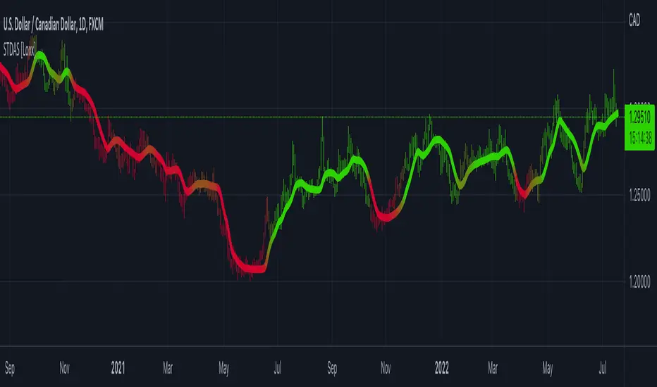
Trend Gradient Moving Average This moving average uses a gradient function which calculates the number of advances/declines of the moving average to change the intensity of the colors, meaning a longer trend in either direction will show a stronger color. You can choose 3 colors to build the gradient: a bullish, bearish & neutral/transition color. The number of steps chosen will change the speed of color change, with a lower number of steps meaning a faster transition and viceversa.
Furthermore, you can choose between many different types of moving averages:
-SMA (Simple Moving Average)
-EMA (Exponential Moving Average)
-RMA (Rolling Moving Average)
-WMA (Weighted Moving Average)
-HMA (Hull Moving Average)
-VWMA (Volume Weighted Moving Average)
-TMA (Triangular Moving Average)
Enjoy!


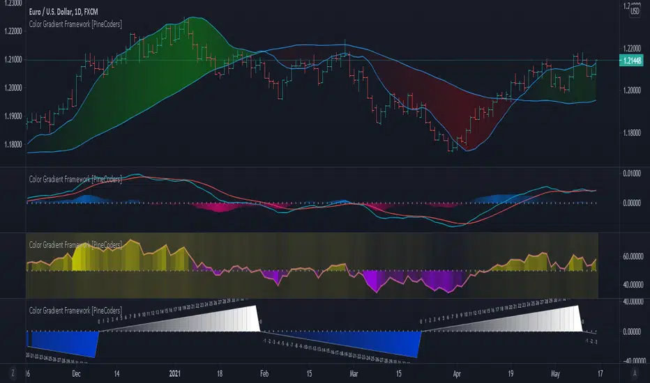
Color Gradient Framework [PineCoders]█ OVERVIEW
This indicator shows how you can use the new color functions in Pine to generate color gradients. We provide functions that will help Pine coders generate gradients for multiple use cases using base colors for bull and bear states.
█ CONCEPTS
For coders interested in maximizing the use of color in their scripts, TradingView has added new color functions and new functionality to existing functions. For us coders, this translates in the ability to generate colors on the fly and use dynamic colors ("series color") in more places.
New functions allow us to:
• Generate colors dynamically from calculated RGBA components ("A" is the Alpha channel, known to Pine coders as the "transparency"). See color.rgb() .
• Extract RGBA components from existing colors. See color.r() , color.g() , color.b() and color.t() .
• Generate linear gradients between two colors. See color.from_gradient() .
Improvements to existing color/plotting functions allow more flexible use of color:
• plotcandle() now accepts a "series color" argument for its `wickcolor` and `bordercolor` parameters.
• plotarrow() now accepts a "series color" argument for its `colorup` and `colordown` parameters.
Gradients are not only useful to make script visuals prettier; they can be used to pack more information in your displays. Our gradient #4 goes overboard with the concept by using a different gradient for the source line, its fill, and the background.
█ OUR SCRIPT
The script presents four functions to generate gradients:
f_c_gradientRelative(_source, _min, _max, _c_bear, _c_bull)
f_c_gradientRelativePro(_source, _min, _max, _c_bearWeak, _c_bearStrong, _c_bullWeak, _c_bullStrong)
f_c_gradientAdvDec(_source, _center, _c_bear, _c_bull)
f_c_gradientAdvDecPro(_source, _center, _steps, _c_bearWeak, _c_bearStrong, _c_bullWeak, _c_bullStrong)
The relative gradient functions are useful to generate gradients on a source that oscillates between known upper/lower limits. They use the relative position of the source between the `_min` and `_max` levels to generate the color. A centerline is derived from the `_min` and `_max` levels. The source's position above/below that centerline determines if the bull/bear color is used, and the relative position of the source between the centerline and the max/min level determines the gradient of the bull/bear color.
The advance/decline gradient functions are useful to generate gradients on a source for which min/max levels are unknown. These functions use source advances and declines to determine a gradient level. The `f_c_gradientAdvDec()` version uses the historical maximum of advances/declines to determine how many correspond to the strongest bull/bear colors, making its gradients adaptive. The `f_c_gradientAdvDecPro()` version requires the explicit number of advances/declines that correspond to the strongest bull/bear colors. This is useful when coloring chart bars, for example, where too many gradient levels are difficult to distinguish. Using the Pro version of the function allows you to limit the number of gradient levels to 5, for example, so that transitions are fewer, but more obvious. The `_center` parameter of the advance/decline functions allows them to determine which of the bull/bear colors to use.
Note that the custom `f_colorNew(_color, _transp)` function we use in our script should soon no longer be necessary, as changes are under way to allow color.new() to accept series arguments.
Inputs
The script's inputs demonstrate one way you can allow users to choose base bull/bear colors. Because users can modify any of the colors, only two are technically needed: one for bull, one for bear, as we do for the configuration of the bull/bear colors for the background in the gradient #4 configuration. Providing a few presets from which users can choose can be useful for color-challenged script users, but that type of inputs has the disadvantage of not rendering optimally in all OS/Browser environments.
You can use the inputs to select one of eight gradient demonstrations to display.
█ THANKS
Thanks to the PineCoders team for validating the code and description of this publication.
Thanks also to the many TradingView devs from multiple teams who made these improvements to Pine colors possible.
Look first. Then leap.
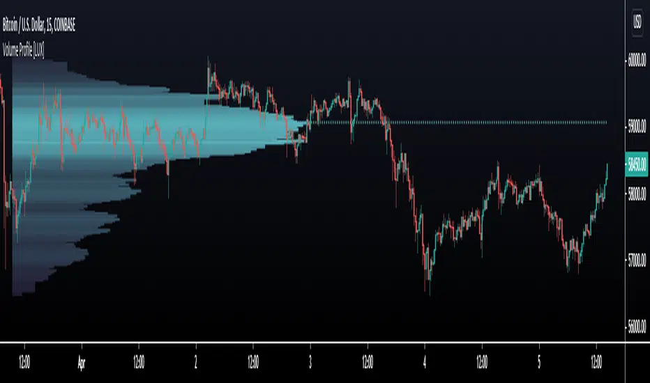
Volume Profile [LuxAlgo]Displays the estimate of a volume profile, with the option to show a rolling POC (point of control). Users can change the lookback, row size, and various visual aspects of the volume profile.
Settings
Basic:
Lookback: Number of most recent bars to use for the calculation of the volume profile
Row Size: Determines the number of rows used for the calculation of the volume profile
Show Rolling POC: Determines whether to display the rolling POC of the volume profile
Style:
Width (% of the box): Determines the length of the bars relative to the Lookback value
Bar Width: Width of each bar
Flip Histogram: Flips the histogram, when enabled, the histogram base will be located at the most recent candle
Gradient: Allows to color the volume profile bars with a gradient, with a color intensity determined by the length of each bar
Rows Solid Color: Color of each bar when 'Gradient' is disabled
POC Solid Color: Color of the POC when 'Gradient' is disabled
Usage
It is very common to display volume over time in order to visualize the trading activity made over a specific candle, however this is not the only way to display volume and it can be interesting to put it in relation with the price, which is what volume profiles do.
Volume profiles are displayed as price relative histograms showing the accumulated volume within certain price areas, the number of areas are determined by the row size of the volume profile. Knowing which price's area accumulated the most volume allow highlighting areas of interest to market participants.
Most accumulated volume will be encountered in zones of equilibrium between buyers and sellers; that is zones of local price stationarity. These zones are highlighted by high volume nodes in the volume profile. Imbalance between buyers and sellers are highlighted by thinner zones of the volume profile.
The price level with the most accumulated volume is highlighted by the "point of control" (POC), displayed by the dotted line in the indicator.
The POC is often considered an important level, commonly used as support/resistance by traders. One can verify the accuracy of this use case by using the rolling POC (assuming one would use the POC over time as SR).
Indicator Limitations
Volume profiles are calculated using tick data, which is not the case of this estimate, as such you won't have an accurate representation of an actual volume profile.
The rolling POC can introduce time outs in the script computation, use lower lookback and row size value to display it.
200 Week Moving Average HeatmapСolors part of the SMA depending on the change in % (delta %) to the previous value. From blue(none to low increase) through green(moderate increase) to red(high increase).

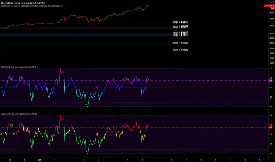
RK's Framework 01 - Auto Color GradientThis started as a personal arrays study, but after a few tests I decided to made a framework to get my own scripts simplest, lighter and faster.
And now I'm sharing with you guys.
Is very simple to use:
Copy evething inside "RK's Auto Color Gradient Framework" block;
Paste anywhere before the plotting;
Declare the color variable name calling the function "f_autocolor(___, ___)" with the source you gonna plot and the size of the scale do you want to use to compare the data.
Feel free to use.
Hope brings some profits for you guys!!
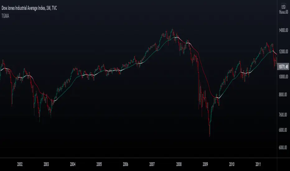
A Useful MA Weighting Function For Controlling Lag & SmoothnessSo far the most widely used moving average with an adjustable weighting function is the Arnaud Legoux moving average (ALMA), who uses a Gaussian function as weighting function. Adjustable weighting functions are useful since they allow us to control characteristics of the moving average such as lag and smoothness.
The following moving average has a simple adjustable weighting function that allows the user to have control over the lag and smoothness of the moving average, we will see that it can also be used to get both an SMA and WMA.
A high-resolution gradient is also used to color the moving average, makes it fun to watch, the plot transition between 200 colors, would be tedious to make but everything was made possible using a custom R script, I only needed to copy and paste the R console output in the Pine editor.
Settings
length : Period of the moving average
-Lag : Setting decreasing the lag of the moving average
+Lag : Setting increasing the lag of the moving average
Estimating Existing Moving Averages
The weighting function of this moving average is derived from the calculation of the beta distribution, advantages of such distribution is that unlike a lot of PDF, the beta distribution is defined within a specific range of values (0,1). Parameters alpha and beta controls the shape of the distribution, with alpha introducing negative skewness and beta introducing positive skewness, while higher values of alpha and beta increase kurtosis.
Here -Lag is directly associated to beta while +Lag is associated with alpha . When alpha = beta = 1 the distribution is uniform, and as such can be used to compute a simple moving average.
Moving average with -Lag = +Lag = 1 , its impulse response is shown below.
It is also possible to get a WMA by increasing -Lag , thus having -Lag = 2 and +Lag = 1 .
Using values of -Lag and +Lag equal to each other allows us to get a symmetrical impulse response, increasing these two values controls the heaviness of the tails of the impulse response.
Here -Lag = +Lag = 3 , note that when the impulse response of a moving average is symmetrical its lag is equal to (length-1)/2 .
As for the gradient, the color is determined by the value of an RSI using the moving average as input.
I don't promise anything but I will try to respond to your comments
