Indicators and strategies
RSI (14) with Auto Zone Colors — Overbought/Oversold HighlighterThis indicator plots the Relative Strength Index (RSI 14) with dynamic color changes for instant visual clarity:
✅ Green line in overbought zone (≥70)
✅ Red line in oversold zone (≤30)
✅ White line in neutral range (30–70)
Includes reference lines at 70, 50, and 30 for quick decision-making. Perfect for spotting momentum extremes, divergences, and potential reversal points without squinting at numbers. Works on any timeframe.

EMA Pullback Entry SignalsEMA Pullback Entry Signals is a tool designed to help traders identify trend continuation opportunities by detecting price pullbacks toward a slow EMA (Exponential Moving Average) during trending conditions.
This indicator combines moving average crossovers, price interaction with EMAs, and optional filtering to improve the timing and quality of trend entries.
Core Features:
Golden Cross / Death Cross Detection
Golden Cross: Fast EMA crossing above Slow EMA
Death Cross: Fast EMA crossing below Slow EMA
Optional X-shaped markers for crossover visualization
Pullback Signal on Slow EMA
Green triangle: Price crosses up through the slow EMA during a bullish trend
Red triangle: Price crosses down through the slow EMA during a bearish trend
Designed to capture continuation entries after a trend pullback
Optional Fast EMA Signals
Green arrow: Price crosses above fast EMA in a bull trend
Red arrow: Price crosses below fast EMA in a bear trend
Helps confirm minor retracements or short-term momentum shifts
Sideways Market Filter
Suppresses signals when the fast and slow EMAs are too close
Prevents entries during low-trend or choppy price action
Cooldown Timer
Enforces a minimum bar interval between signals to reduce overtrading
Helps avoid multiple entries from clustered signals
Custom Alerts
Alerts available for all signal types
Include ticker and timeframe in each alert message
Configurable Settings:
Fast and slow EMA lengths1
Toggle individual signal types (pullbacks, fast EMA crosses, crossovers)
Enable/disable cooldown logic and set bar duration
Sideways market detection sensitivity (EMA proximity threshold)
Primary Use Case
This script is most useful for trend-following traders seeking to enter pullbacks after a trend is established. When the price retraces to the slow EMA and then resumes in the trend direction, it can offer high-quality continuation setups. Works well across timeframes and markets.

Equilibrium TrackerWhat does this indicator do?
This is a screener that checks if the current HTF High moves above the previous HTF High.
This also applies for the low moving below the previous low.
If the 50% of the previous candle is touched, this wil also show in the table and send alerts.
Features
Select up to 2 timeframes and 10 instruments.
A screener table will show all instruments and will light up if an event occurs
Alerts can also get fired
Usage:
Select a chart for example 1 minute
Configure the indicator
Create a new alert on the indicator using the lower timeframe chart

ORB 15m – First 15min Breakout (Long/Short)ORB 15m – First 15min Breakout (Long/Short)
Apply on SPY, great returns

Inverted Hammer w/ Buy Signal This indicator will identify inverted hammer candles in a downtrend and also provide a buy signal when the following candle closes above the top wick of the previous inverted hammer candle.
Institutional Momentum Zones (ADX+ROC+DI+MACD+Filters)Institutional Momentum Zones (ADX + ROC + DI + MACD + Filters)
This indicator is designed to help traders visually identify Bullish, Neutral, and Bearish momentum zones on Nifty, indices, or any liquid asset, using a rules-based, institutional-style approach.
It combines multiple professional-grade momentum and trend filters into a single framework:
ADX (Average Directional Index) – Measures trend strength, filters out choppy conditions.
Directional Indicators (+DI / –DI) – Confirms whether bulls or bears are in control.
ROC (Rate of Change) – Quantifies momentum speed and direction.
MACD (optional) – Adds confirmation by checking multi-timeframe momentum alignment.
EMA Filters (optional) – Ensures price is in alignment with long-term trend bias.
Supertrend (optional) – Can be enabled for additional trend confirmation.
How it works:
Bullish Zone (Green) → Strong trend (ADX > threshold) + upward momentum (ROC > 0, +DI > –DI) + optional EMA/MACD/Supertrend confirmation.
Bearish Zone (Red) → Strong trend (ADX > threshold) + downward momentum (ROC < 0, –DI > +DI) + optional EMA/MACD/Supertrend confirmation.
Neutral Zone (Yellow) → Low trend strength (ADX < threshold) or mixed momentum signals.
Features:
Automatic background coloring for zone detection.
On-chart labels marking new zone changes.
EMA50 / EMA200 and Supertrend overlay options.
Signal markers for bullish/bearish entries.
Info panel with live ADX, ROC, DI values, and MACD histogram.
Alert conditions for zone changes (Bull, Bear, Neutral).
Best used for:
Index momentum tracking (e.g., Nifty, Bank Nifty, Dow, S&P500)
Swing trading & positional trading strategies
Filtering trades to avoid entering during low-momentum chop
Tip: For Nifty positional trading, use Daily or 4H charts with EMA & MACD filters enabled for cleaner, high-confidence signals.

Mutanabby_AI | Fresh Algo V24Mutanabby_AI | Fresh Algo V24: Advanced Multi-Mode Trading System
Overview
The Mutanabby_AI Fresh Algo V24 represents a sophisticated evolution of multi-component trading systems that adapts to various market conditions through advanced operational configurations and enhanced analytical capabilities. This comprehensive indicator provides traders with multiple signal generation approaches, specialized assistant functions, and dynamic risk management tools designed for professional market analysis across diverse trading environments.
Primary Signal Generation Framework
The Fresh Algo V24 operates through two fundamental signal generation approaches that accommodate different market perspectives and trading philosophies. The Trending Signals Mode serves as the primary trend-following mechanism, combining Wave Trend Oscillator analysis with Supertrend directional signals and Squeeze Momentum breakout detection. This mode incorporates ADX filtering that requires values exceeding 20 to ensure sufficient trend strength exists before signal activation, making it particularly effective during sustained directional market movements where momentum persistence creates profitable trading opportunities.
The Contrarian Signals Mode provides an alternative approach targeting reversal opportunities through extreme market condition identification. This mode activates when the Wave Trend Oscillator reaches critical threshold levels, specifically when readings surpass 65 indicating potential bearish reversal conditions or drop below 35 suggesting bullish reversal opportunities. This methodology proves valuable during overextended market phases where mean reversion becomes statistically probable.
Advanced Filtering Mechanisms
The system incorporates multiple sophisticated filtering mechanisms designed to enhance signal quality and reduce false positive occurrences. The High Volume Filter requires volume expansion confirmation before signal activation, utilizing exponential moving average calculations to ensure institutional participation accompanies price movements. This filter substantially improves signal reliability by eliminating low-conviction breakouts that lack adequate volume support from professional market participants.
The Strong Filter provides additional trend confirmation through 200-period exponential moving average analysis. Long position signals require price action above this benchmark level, while short position signals necessitate price action below it. This ensures strategic alignment with longer-term trend direction and reduces the probability of trading against major market movements that could invalidate shorter-term signals.
Cloud Filter Configuration System
The Fresh Algo V24 offers four distinct cloud filter configurations, each optimized for specific trading timeframes and market approaches. The Smooth Cloud Filter utilizes the mathematical relationship between 150-period and 250-period exponential moving averages, providing stable trend identification suitable for position trading strategies. This configuration generates signals exclusively when price action aligns with cloud direction, creating a more deliberate but highly reliable signal generation process.
The Swing Cloud Filter employs modified Supertrend calculations with parameters specifically optimized for swing trading timeframes. This filter achieves optimal balance between responsiveness and stability, adapting effectively to medium-term price movements while filtering excessive market noise that typically affects shorter-term analytical systems.
For active intraday traders, the Scalping Cloud Filter utilizes accelerated Supertrend calculations designed to capture rapid trend changes effectively. This configuration provides enhanced signal generation frequency suitable for compressed timeframe strategies. The advanced Scalping+ Cloud Filter incorporates Hull Moving Average confirmation, delivering maximum responsiveness for ultra-short-term trading while maintaining signal quality through additional momentum validation processes.
Specialized Assistant Functionality
The system includes two distinct assistant modes that provide supplementary market analysis capabilities. The Trend Assistant Mode activates advanced cloud analysis overlays that display dynamic support and resistance zones calculated through adaptive volatility algorithms. These levels automatically adjust to current market conditions, providing visual guidance for identifying trend continuation patterns and potential reversal areas with mathematical precision.
The Trend Tracker Mode concentrates on long-term trend identification by displaying major exponential moving averages with color-coded fill areas that clarify directional bias. This mode maintains visual simplicity while providing comprehensive trend context evaluation, enabling traders to quickly assess broader market direction and align shorter-term strategies accordingly.
Dynamic Risk Management System
The integrated risk management system automatically adapts across all operational modes, calculating stop loss and take profit targets using Average True Range multiples that adjust to current market volatility. This approach ensures consistent risk parameters regardless of selected operational mode while maintaining relevance to prevailing market conditions.
Stop loss placement occurs at dynamically calculated distances from entry points, while three progressive take profit targets establish at customizable ATR multiples respectively. The system automatically updates these levels upon trend direction changes, ensuring current market volatility influences all risk calculations and maintains appropriate risk-reward ratios throughout trade management.
Comprehensive Market Analysis Dashboard
The sophisticated dashboard provides real-time market analysis including volatility measurements, institutional activity assessment, and multi-timeframe trend evaluation across five-minute through four-hour periods. This comprehensive market context assists traders in selecting appropriate operational modes based on current market characteristics rather than relying exclusively on historical performance data.
The multi-timeframe analysis ensures mode selection considers broader market context beyond the primary trading timeframe, improving overall strategic alignment and reducing conflicts between different temporal market perspectives. The dashboard displays market state classification, volatility percentages, institutional activity levels, current trading session information, and trend pressure indicators with professional formatting and clear visual hierarchy.
Enhanced Trading Assistants
The Fresh Algo V24 includes specialized trading assistant features that complement the primary signal generation system. The Reversal Dot functionality identifies potential reversal points through Wave Trend Oscillator analysis, displaying visual indicators when crossover conditions occur at extreme levels. These reversal indicators provide early warning signals for potential trend changes before they appear in the primary signal system.
The Dynamic Take Profit Labels feature automatically identifies optimal profit-taking opportunities through RSI threshold analysis, marking potential exit points at multiple levels for long positions and corresponding levels for short positions. This automated profit management system helps traders optimize exit timing without requiring constant manual monitoring of technical indicators.
Advanced Alert System
The comprehensive alert system accommodates all operational modes while providing granular notification control for various signal types and risk management events. Traders can configure separate alerts for normal buy signals, strong buy signals, normal sell signals, strong sell signals, stop loss triggers, and individual take profit target achievements.
Cloud crossover alerts notify traders when trend direction changes occur, providing early indication of potential strategy adjustments. The alert system includes detailed trade setup information, timeframe data, and relevant entry and exit levels, ensuring traders receive complete context for informed decision-making without requiring constant chart monitoring.
Technical Foundation Architecture
The Fresh Algo V24 combines multiple proven technical analysis components including Wave Trend Oscillator for momentum assessment, Supertrend for directional bias determination, Squeeze Momentum for volatility analysis, and various exponential moving averages for trend confirmation. Each component contributes specific market insights while the unified system provides comprehensive market evaluation through their mathematical integration.
The multi-component approach reduces dependency on individual indicator limitations while leveraging the analytical strengths of each technical tool. This creates a robust analytical framework capable of adapting to diverse market conditions through appropriate mode selection and parameter optimization, ensuring consistent performance across varying market environments.
Market State Classification
The indicator incorporates advanced market state classification through ADX analysis, distinguishing between trending, ranging, and transitional market conditions. This classification system automatically adjusts signal sensitivity and filtering parameters based on current market characteristics, optimizing performance for prevailing conditions rather than applying static analytical approaches.
The volatility measurement system calculates current market activity levels as percentages, providing quantitative assessment of market energy and helping traders select appropriate operational modes. Institutional activity detection through volume analysis ensures signal generation aligns with professional market participation patterns.
Implementation Strategy Considerations
Successful implementation requires careful matching of operational modes to prevailing market conditions and individual trading objectives. Trending modes demonstrate optimal performance during directional markets with sustained momentum characteristics, while contrarian modes excel during range-bound or overextended market conditions where reversal probability increases.
The cloud filter configurations provide varying degrees of confirmation strength, with smoother settings reducing false signal occurrence at the expense of some responsiveness to price changes. Traders must balance signal quality against signal frequency based on their risk tolerance and available trading time, utilizing the comprehensive customization options to optimize performance for their specific requirements.
Multi-Timeframe Integration
The system provides seamless multi-timeframe analysis through the integrated dashboard, displaying trend alignment across multiple time horizons from five-minute through four-hour periods. This analysis helps traders understand broader market context and avoid conflicts between different temporal perspectives that could compromise trade outcomes.
Session analysis identifies current trading session characteristics, providing context for expected market behavior patterns and helping traders adjust their approach based on typical session volatility and participation levels. This geographic market awareness enhances strategic decision-making and improves timing for trade execution.
Advanced Visualization Features
The indicator includes sophisticated visualization capabilities through gradient candle coloring based on MACD analysis, providing immediate visual feedback on momentum strength and direction. This enhancement allows rapid market assessment without requiring detailed indicator analysis, improving efficiency for traders managing multiple instruments simultaneously.
The cloud visualization system uses color-coded fill areas to clearly indicate trend direction and strength, with automatic adaptation to selected operational modes. This visual clarity reduces analytical complexity while maintaining comprehensive market information display through professional chart presentation.
Performance Optimization Framework
The Fresh Algo V24 incorporates performance optimization features including signal strength classification, automatic parameter adjustment based on market conditions, and dynamic filtering that adapts to current volatility levels. These optimizations ensure consistent performance across varying market environments while maintaining signal quality standards.
The system automatically adjusts sensitivity levels based on selected operational modes, ensuring appropriate responsiveness for different trading approaches. This adaptive framework reduces the need for manual parameter adjustments while maintaining optimal performance characteristics for each operational configuration.
Conclusion
The Mutanabby_AI Fresh Algo V24 represents a comprehensive solution for professional trading analysis, combining multiple analytical approaches with advanced visualization and risk management capabilities. The system's strength lies in its adaptive multi-mode design and sophisticated filtering mechanisms, providing traders with versatile tools for various market conditions and trading styles.
Success with this system requires understanding the relationship between different operational modes and their optimal application scenarios. The comprehensive dashboard and alert system provide essential market context and trade management support, enabling systematic approach to market analysis while maintaining flexibility for individual trading preferences.
The indicator's sophisticated architecture and extensive customization options make it suitable for traders at all experience levels, from those seeking systematic signal generation to advanced practitioners requiring comprehensive market analysis tools. The multi-timeframe integration and adaptive filtering ensure consistent performance across diverse market conditions while providing clear guidelines for strategic implementation.

Ichimoku + Daily-Candle_X + HULL-MA_X + MacD Here’s a clean and clear **description** you can use for your **"Ichimoku + Daily-Candle\_X + HULL-MA\_X + MacD"** strategy in Pine Script or documentation:
📈 **Strategy Description: Ichimoku + Daily-Candle\_X + HULL-MA\_X + MacD**
This multi-factor trading strategy combines **trend**, **momentum**, and **price confirmation** indicators to generate high-confluence entry signals. It’s designed for traders seeking precision entries based on multiple layers of confirmation across different timeframes.
🔍 **Core Components**
1. **Ichimoku Cloud (Trend Confirmation)**
* Uses **Tenkan-sen (Conversion Line)**, **Kijun-sen (Base Line)**, and **Senkou Spans A & B**.
* Confirms long bias when **Leading Span A > B**, and short bias when **Span A < B**.
2. **Daily Candle Cross (Multi-Timeframe Price Action)**
* Compares the **current daily candle price** with the previous.
* Bullish if today's price > yesterday’s; bearish if lower.
* Adds higher-timeframe momentum context.
3. **Double Hull Moving Average Cross**
* Uses a fast-reacting **Hull MA** on the current and previous bars.
* A bullish signal triggers when current HMA > previous HMA (trend strength).
* Smooths out price noise better than traditional MAs.
4. **Custom Hull-Based MACD (Momentum)**
* Calculates the MACD line using **two Hull MAs** (fast and slow).
* Signal line is another Hull MA of the MACD.
* A bullish signal is when **MACD > Signal Line**, bearish when the opposite.
---
📌 **Entry Conditions*
*Long Entry*
* HMA cross is bullish
* Daily candle momentum is up
* Price is above previous HMA
* Ichimoku cloud shows bullish trend
* MACD is above its signal line
*Short Entry**
* All above conditions flipped for bearish signals
🧠 **Strategy Objective**
This strategy aims to:
* Filter out false signals by requiring multiple confirmations
* Catch **sustained directional trends** instead of short-term fluctuations
* Use higher timeframe context (daily candles) for better reliability

Sigma Expected Movement [D/W/M] - Jez WhitakerThis indicator aims to help those with lower levels of TradingView add day trading indicators without going over their limits. You can toggle on and off the indicators you want and change the settings but you should see:
MAs - 5, 20, 50, 100, 200
VWAPS - daily, WTD, MTD, YTD
Previous close, previous highs, previous lows etc.

Tabela RSI e Tendência EMA MTF - 2This custom TradingView indicator provides a consolidated view of trend and Relative Strength Index (RSI) across multiple timeframes, all within an intuitive table directly on your chart. Designed for traders seeking quick and efficient analysis of market momentum and direction across different time horizons, this indicator automatically adapts to the asset you are currently viewing.

UNITY[ALGO] PO3 V3Of course. Here is a complete and professional description in English for the indicator we have built, detailing all of its features and functionalities.
Indicator: UNITY PO3 V7.2
Overview
The UNITY PO3 is an advanced, multi-faceted technical analysis tool designed to identify high-probability reversal setups based on the Swing Failure Pattern (SFP). It combines real-time SFP detection on the current timeframe with a sophisticated analysis of key institutional liquidity zones from the H4 timeframe, presenting all information in a clear, dynamic, and interactive visual interface.
This indicator is built for traders who use liquidity concepts, providing a complete dashboard of entries, targets, and invalidation levels directly on the chart.
Core Features & Functionality
1. Swing Failure Pattern (SFP) Detection (Current Timeframe)
The indicator's primary engine identifies SFPs on the chart's active timeframe with two layers of logic:
Standard SFP: Detects a classic liquidity sweep where the current candle's wick takes out the high or low of the previous candle and the body closes back within the previous candle's range.
Outside Bar SFP Logic: Intelligently analyzes engulfing candles that sweep both the high and low of the previous candle. A valid signal is only generated if the candle has a clear directional close:
Bullish Signal: If the outside bar closes higher than its open.
Bearish Signal: If the outside bar closes lower than its open.
Neutral (doji-like) outside bars are ignored to filter for indecision.
2. Comprehensive On-Chart SFP Markings
When a valid SFP is detected, a full suite of dynamic drawings appears on the chart:
Failure Line: A dashed line (red for bearish, green for bullish) marking the precise price level of the liquidity sweep.
PREMIUM ZONE (SFP Candle Wick): A transparent, colored rectangle highlighting the rejection wick of the signal candle (the upper wick for bearish SFPs, the lower wick for bullish SFPs). This zone automatically extends to the right, following the current price, until the DOL is hit.
CRT BOX (Reference Candle): A transparent box with a colored border drawn around the entire range of the candle that was swept (Candle 1). This highlights the full liquidity zone and also extends dynamically until the DOL is hit.
Dynamic Target Line: A blue dashed line marking the primary objective (the low of the signal candle for shorts, the high for longs).
The line begins with a "⏳ Target" label and extends with the current price.
Upon being touched by price, the line freezes, and its label permanently changes to "✅ Target".
Dynamic DOL (Draw on Liquidity) Line: An orange dashed line marking the invalidation level, defined as the opposite extremity of the swept candle (Candle 1).
It begins with a "⏳ dol" label and extends with the price.
Upon being touched, it freezes, and its label changes to "✅ dol".
3. Multi-Session Killzone Liquidity Levels (H4 Analysis)
The indicator automatically analyzes the H4 timeframe in the background to identify and plot key liquidity levels from three major trading sessions, based on their UTC opening times.
1am Killzone (London Lunch): Tracks the high/low of the 05:00 UTC H4 candle.
5am Killzone (London Open): Tracks the high/low of the 09:00 UTC H4 candle.
9am Killzone (NY Open): Tracks the high/low of the 13:00 UTC H4 candle.
For each of these Killzones, the indicator provides two types of analysis:
Last KZ Lines: Plots the high and low of the most recent qualifying Killzone candle. These lines are dynamic, extending with price and showing a ⏳/✅ status when touched.
Fresh Zones: A powerful feature that scans the entire available history of Killzones to find and display the closest untouched high (above the current price) and the closest untouched low (below the current price). These "Fresh" lines are also fully dynamic and provide a real-time view of the most relevant nearby liquidity targets.
4. Advanced User Settings & Chart Management
The indicator is designed for a clean and user-centric experience with powerful customization:
Show Only Last SFP: Keeps the chart clean by automatically deleting the previous SFP setup when a new one appears.
Hide SFP on DOL Reset: When checked, automatically removes all drawings related to an SFP setup the moment its invalidation level (DOL line) is touched. This leaves only active, valid setups on the chart.
Hide Consumed KZ: When checked, automatically removes any Killzone or Fresh Zone line from the chart as soon as it is touched by the price.
Independent Toggles: Every visual element—SFP signals, each of the three Killzones, and their respective "Fresh" zone counterparts—can be turned on or off independently from the settings menu for complete control over the visual display.
Z-Order Priority: All indicator drawings are rendered in front of the chart candles, ensuring they are always clearly visible and never hidden from view.
Average VolatilityThis script offers a unique and practical approach to visualizing average volatility by calculating a simple moving average of the daily high-low ranges, directly reflecting price fluctuations over a user-defined period. Unlike standard volatility indicators, it provides customizable options such as adjustable period length, display of absolute and percentage volatility values, and flexible text formatting for clear and tailored insights. This makes it a valuable tool for traders seeking to better understand market volatility trends and manage risk more effectively. Its straightforward visualization supports informed decision-making across various instruments and timeframes.
The indicator displays the average volatility over a configurable period as a bar chart (originally designed for daily intervals). It visualizes the price range (difference between high and low) across a selectable number of periods, as well as its ratio to the closing price, offering various customization options.
For many traders, assets with daily moves of 1% or more may offer greater profit opportunities, especially for short-term trading strategies. Instruments with lower volatility are generally less favored and often not recommended in such approaches due to reduced trading potential. Please note that higher volatility also implies increased risk, and potential losses can be significant. Always use proper risk management.
Detailed description:
The script calculates average volatility as a simple moving average of the high-low ranges (default: 5 periods, intended for daily timeframes). Volatility can be shown as either a bar or line chart. Users can choose to display the absolute volatility values and/or the volatility expressed as a percentage of the closing price. Text size and spacing between labels are adjustable to ensure readability across different instruments. Additionally, the last (unconfirmed) bar can be shown or hidden, since its value depends on the current price. Overall, the script provides a flexible and clear visualization of an instrument’s volatility.
---
Russian:
Индикатор отображает среднюю волатильность как простое скользящее среднее диапазонов «максимум-минимум» (по умолчанию 5 периодов, предназначено для дневных таймфреймов). Волатильность может отображаться в виде столбчатой или линейной диаграммы. Пользователи могут выбрать отображение абсолютных значений волатильности и/или волатильности, выраженной в процентах от цены закрытия. Размер текста и расстояния между надписями регулируются для удобочитаемости на разных инструментах. Кроме того, последний (неподтверждённый) столбец можно показать или скрыть, так как его значение зависит от текущей цены. В общем, скрипт обеспечивает гибкое и наглядное отображение волатильности инструмента.
Активы с волатильностью от 1% и выше дают больше возможностей для краткосрочной торговли, но риск также выше. Инструменты с низкой волатильностью не рекомендуются для таких подходов из-за ограниченного торгового потенциала и сложности в реализации прибыльных сделок. Всегда применяйте риск-менеджмент.
---
Spanish:
El script calcula la volatilidad promedio como un promedio móvil simple de las diferencias entre máximos y mínimos (por defecto 5 periodos, pensado para intervalos diarios). La volatilidad puede mostrarse como gráfico de barras o de líneas. El usuario puede elegir mostrar los valores absolutos de la volatilidad y/o los valores expresados en porcentaje respecto al precio de cierre. El tamaño del texto y el espacio entre las etiquetas son ajustables para garantizar la legibilidad en diferentes instrumentos. Además, se puede mostrar u ocultar la última barra (no confirmada), ya que su valor depende del precio actual. En conjunto, el script proporciona una visualización flexible y clara de la volatilidad del instrumento.
Los activos con una volatilidad del 1% o más ofrecen mayores oportunidades para el trading a corto plazo, pero también conllevan un mayor riesgo. Los instrumentos con baja volatilidad no se recomiendan para este tipo de estrategias debido a su limitado potencial de trading y la dificultad para obtener ganancias. Siempre utilice una gestión de riesgos adecuada.

Position Sizing Risk TablePosition Sizing Risk Table - swing trading. Allowing for a 0,25; 0,5 and 1% risk based on NAV

Index Contracts Calculator (NQ/ES) — Label"Quick micro futures position size calculator for NQ and ES. Enter risk in dollars and stop size in points, and it instantly shows how many contracts you can take — right on your chart."

ORB Scalp setup on 15min by UnenbatThis indicator draws a 2-minute Opening Range Box (ORB) at the beginning of each 15-minute candle by combining the last minute of the previous candle and the first minute of the current one. It highlights the session high/low during this range, and extends the box for a customizable duration. TP and BE lines are also plotted above/below the range for strategic planning. Perfect for scalpers using 15-minute timeframe.

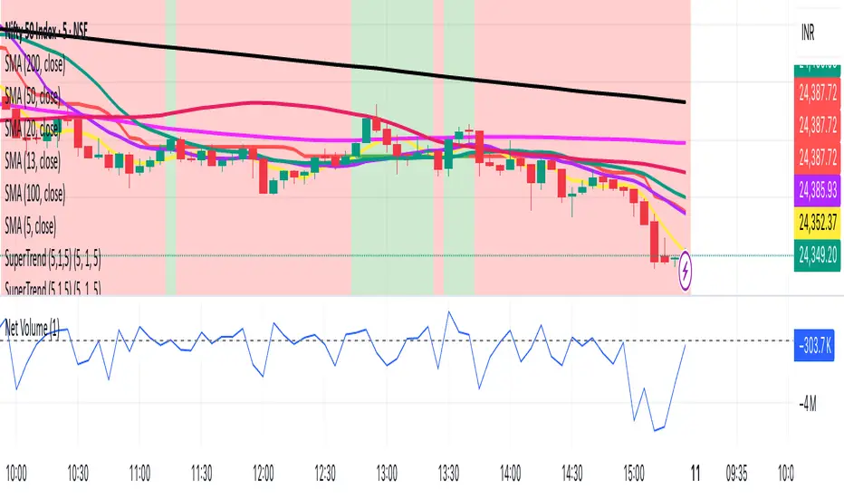
SuperTrend (5,1,5) By satish SWhy 3 Supertrends?
Short-term Supertrend (7, 1, 3) → reacts quickly, catches early trend changes but can give more false signals.
Medium-term Supertrend (14, 1, 2) → smoother, filters out noise.
Long-term Supertrend (21, 1, 3) → confirms major trend direction, fewer whipsaws.
How it Works
Trend Reversal Detection
If all three flip in the same direction → strong confirmation of trend change.
If only the short-term flips but others don’t → possible false signal, wait for confirmation.
Entry Signal Example
Buy when all three turn green (Supertrend below price).
Sell/short when all three turn red (Supertrend above price).
Exit / Partial Profit
Exit when the shortest one (7, 1, 3) flips against your position — protects profits in choppy markets.
TradingView Setup
You can do this by:
Adding Supertrend three times.
Setting their (Period, Multiplier, ATR Type) to:
ST1: 7, 1, 3
ST2: 14, 1, 2
ST3: 21, 1, 3
Use different colors or line styles for each so you can spot alignment quickly.
SuperTrend (5,1,5) BY Satish SWhy 3 Supertrends?
Short-term Supertrend (7, 1, 3) → reacts quickly, catches early trend changes but can give more false signals.
Medium-term Supertrend (14, 1, 2) → smoother, filters out noise.
Long-term Supertrend (21, 1, 3) → confirms major trend direction, fewer whipsaws.
How it Works
Trend Reversal Detection
If all three flip in the same direction → strong confirmation of trend change.
If only the short-term flips but others don’t → possible false signal, wait for confirmation.
Entry Signal Example
Buy when all three turn green (Supertrend below price).
Sell/short when all three turn red (Supertrend above price).
Exit / Partial Profit
Exit when the shortest one (7, 1, 3) flips against your position — protects profits in choppy markets.
TradingView Setup
You can do this by:
Adding Supertrend three times.
Setting their (Period, Multiplier, ATR Type) to:
ST1: 7, 1, 3
ST2: 14, 1, 2
ST3: 21, 1, 3
Use different colors or line styles for each so you can spot alignment quickly.

SuperTrend with 3 Inputs SatishWhy 3 Supertrends?
Short-term Supertrend (7, 1, 3) → reacts quickly, catches early trend changes but can give more false signals.
Medium-term Supertrend (14, 1, 2) → smoother, filters out noise.
Long-term Supertrend (21, 1, 3) → confirms major trend direction, fewer whipsaws.
How it Works
Trend Reversal Detection
If all three flip in the same direction → strong confirmation of trend change.
If only the short-term flips but others don’t → possible false signal, wait for confirmation.
Entry Signal Example
Buy when all three turn green (Supertrend below price).
Sell/short when all three turn red (Supertrend above price).
Exit / Partial Profit
Exit when the shortest one (7, 1, 3) flips against your position — protects profits in choppy markets.
TradingView Setup
You can do this by:
Adding Supertrend three times.
Setting their (Period, Multiplier, ATR Type) to:
ST1: 7, 1, 3
ST2: 14, 1, 2
ST3: 21, 1, 3
Use different colors or line styles for each so you can spot alignment quickly.

💎 ENJOYBLUE ⏰ Open Price AlertThis Pine Script (version 6) is designed for TradingView to monitor the closing of a user-selected Timeframe (TF) — for example, M30, H1, H4, or D1 — and trigger an alert immediately when that TF’s candle closes. Along with the alert, it displays the current open prices from four higher-level timeframes:
Open MN: Open price of the current monthly candle
Open W1: Open price of the current weekly candle
Open D1: Open price of the current daily candle
Open H4: Open price of the current 4-hour candle
The alert message is formatted into a single compact line to ensure it is fully visible on mobile devices!
~ENJOYBLUE 💎
