Predictive Ranges [LuxAlgo]The Predictive Ranges indicator aims to efficiently predict future trading ranges in real-time, providing multiple effective support & resistance levels as well as indications of the current trend direction.
Predictive Ranges was a premium feature originally released by LuxAlgo in 2020.
The feature was discontinued & made legacy, however, due to its popularity and reproduction attempts, we deemed it necessary to release it open source to the community.
🔶 USAGE
The primary purpose of this indicator is to provide potential support & resistance levels on the chart by estimating future trading ranges.
When the price reaches one of the upper/lower levels of the Predictive Ranges we can expect the price to reverse.
If the price exits the predicted range, new levels are given in real-time & they do not repaint. Higher "Factor" values allow returning longer term and wider ranges less susceptible to be exited.
🔹 Estimating Trend Directions
Users are able to easily estimate trend directions by looking at the central levels of the predictive ranges, which represent an estimate of the price central tendency.
If this central level increases it means the price is up-trending, if it is decreasing price is down-trending.
🔶 SETTINGS
Length: ATR Length used for the indicator calculation. Higher values will tend to return ranges of equal width.
Factor: Control the ranges width. Higher values will return less frequent ranges, each having a higher width.
Timeframe: Indicator timeframe output.
Source: Input source of the indicator. It is recommended to use input sources on the same scale as the price.
Prediction

Monte Carlo Price ProbabilitiesMonte Carlo simulations have been a popular tool in the world of finance, risk analysis, and decision making for decades. In this post, I will take you through the history of Monte Carlo simulations and explain how I implemented this powerful technique in Pine Script. This implementation can help traders and investors in various time frames to better understand the potential future price movements of financial instruments based on historical data.
History of Monte Carlo Simulations
The Monte Carlo method was named after the famous Monte Carlo Casino in Monaco, as the technique involves using random sampling to approximate solutions to mathematical problems. The method was first introduced by Stanislaw Ulam, a mathematician working on the Manhattan Project in the 1940s. Ulam realized that using random sampling could provide approximate solutions to complex problems that were otherwise difficult or impossible to solve analytically.
Over the years, Monte Carlo simulations have found applications in various fields, including physics, engineering, and finance. In the world of finance, the method has been used to model stock price movements, option pricing, portfolio optimization, and risk management.
Implementation in Pine
In my implementation of Monte Carlo simulations in Pine, I created a script that allows users to input several parameters such as the arbitrary price, number of simulations, number of steps into the future, and the start bar index. The start bar index is a crucial setting for running the script on lower time frames, as it helps to ensure that the script runs smoothly for a given symbol.
The script then calculates the log return of each bar and categorizes them into green (positive) or red (negative) moves. It uses these historical price movements to calculate the probabilities of future price movements for each step in the simulation.
The core of the Monte Carlo simulation lies in the `monte()` function, which generates random numbers to determine if the next price movement will be green or red, and then selects a move size based on its probability. The `sim()` function runs multiple simulations using the `monte()` function and stores the results in an array.
Finally, the script calculates the probability of the arbitrary price being reached in the future based on the results of the simulations. It also plots the probability on the chart, allowing users to visually assess the potential future price movements of the financial instrument.
Using the Monte Carlo Simulation
To use the Monte Carlo simulation in Pine, you need to input the desired parameters such as the arbitrary price, number of simulations, number of steps into the future, and the start bar index. For some symbols, you may need to set the start bar index to around 10k to ensure that the script runs smoothly.
Once you have input the parameters and run the script, you will see the probability of reaching the arbitrary price plotted on the chart. This can provide a valuable insight into the potential future price movements of the financial instrument based on historical data, helping you make more informed trading and investment decisions.
Conclusion
Monte Carlo simulations have a rich history and have proven to be a valuable tool in various fields, including finance. My implementation of Monte Carlo simulations in Pine allows traders and investors to better understand the potential future price movements of financial instruments in various time frames. By evaluating the probabilities of reaching specific price levels, users can make more informed decisions and better manage their risk.

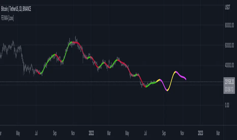
Acceleration-Based MA Slope PredictionHello traders,
I developed this indicator while working on a trading strategy using moving average slope and acceleration, and I found the concept interesting enough to share it.
Let me briefly explain this indicator.
----About White Plot----
1. Calculate the first derivative approximation at the current point of the Moving Average, and then calculate the second derivative approximation to obtain the 'Acceleration'.
2. Where the acceleration is 0, it signifies a change in the force of the moving average.
3. Therefore, by drawing a parabola based on the acceleration at that time, can depict the parabolic shape of the moving average.
This is represented as a white circle on the indicator.
4. These circles are reset at the next point where the acceleration is 0, indicating a change in the parabolic force.
If the moving average rises more sharply than the predicted value of the rising parabola, a more drastic increase is expected.
5. In this case, you can start risk management around the time the drawn parabola breaks.
(The actual MA is represented by green/red lines)
6. Before the trend changes, i.e., before the direction of the moving average changes, there is a section where the acceleration is 0, and this is represented on the chart as follows.
(The lower indicator shows the acceleration of the corresponding parabola)
----About Red Plot----
1. Calculate the first derivative approximation of the moving average value, the 'slope'.
2. Where the slope is 0, it represents the extreme point of the parabola.
3. Therefore, by using the acceleration at that point as the coefficient of the quadratic function and setting the extreme point as a vertex, we can draw a quadratic function. This is represented as a red circle on the indicator.
(Keep in mind that the actual moving average is not a quadratic function; this is a "forced" quadratic function assuming the parabola is maintained)
4. These circles are reset at the next extreme point where the slope is 0, and a new quadratic function is created.
Based on the formula obtained in the above process, you can predict the future moving average through 'offset'.
5. That is, if the x value at the current point is 'k', you can predict the moving average one candle ahead by substituting (k+1) into the quadratic function.
The predicted value at the past position is shown as a red circle.
6. The smoother the chosen moving average, the fewer extreme points will appear, and the higher the likelihood of the parabola fitting.
For the T3 set as the default value, it shows very high accuracy even when predicting about 20 candles ahead.
On the other hand, rough moving averages like SMA have limited prediction value.
(SMA 60, offset = 10)
--------
The moving average with a very high level of accuracy is JMA (Jurik Moving Average). However, since the code for this moving average is not public, I recommend those interested to check it through my code.
Additionally, I believe the code of this indicator I've uploaded has significant utility.
As an example, you can use the breaking point of the parabola predicted by the acceleration to determine when the force changes again for entries/losses. There are many other possible applications as well.
I look forward to seeing more excellent results from this indicator.
--------
안녕하세요 트레이더여러분.
이 지표는, 제가 이동평균선의 기울기와 가속도를 이용하여 매매를 하기 위한 지표를 개발하다가, 흥미로운 내용이라고 판단하여 만들게 되었습니다.
이 지표에 대해 간단히 설명드리겠습니다.
----하얀색 플롯에 대해----
1. 이동평균선이 진행되는 현재 시점에서 미분의 근사값을 구하고, 다시 한 번 미분의 근사값을 구해서 '가속도'를 얻습니다.
2. 가속도가 0이 되는 곳은, 곧 해당 이동평균선의 힘이 바뀌는 곳을 의미합니다.
3. 따라서, 그 당시 시점 기준으로 포물선을 그려낸다면, 가속도를 이용하여 해당 이동평균선의 포물선을 그려낼 수 있습니다. 이것은 지표의 하얀색점로서 표기됩니다.
4. 이 때, 이러한 점들은 다음의 가속도가 0이 되는 지점, 즉 포물선의 힘이 바뀌는 곳에서 다시 초기화됩니다.
5. 올라가고 있던 포물선에서의 예측치보다 이동평균선이 더 급하게 올라간다면, 더욱 급격한 상승이 예상됩니다. 이 경우, 그려지고있는 포물선이 깨질 때쯤부터 리스크 관리를 시작할 수 있습니다.
(녹색/빨간색의 선으로 실제 MA를 표현했습니다. 거슬리시면 '모습'가셔서 끄셔도 좋습니다. )
6. 추세가 변경되기 전, 즉 이동평균선의 방향이 바뀌기 전에는 가속도가 0이 되는 구간이 존재하고, 그것이 차트 위에 다음과같이 표현됩니다.
(하단의 지표는, 해당 포물선의 가속도을 나타냅니다)
----붉은색 플롯에 대해----
1. 이동평균선 값을 미분 근사값 즉, '기울기'를 구합니다.
2. 기울기가 0이 되는 곳은, 포물선이 극점이 되는 곳을 뜻합니다.
3. 따라서, 해당 시점의 가속도를 2차함수의 계수로 하여, 또한 해당 극점을 하나의 꼭지점으로 설정하여,이차함수를 그려낼 수 있습니다. 이것은 지표의 빨간색점으로서 표현됩니다.
(실제 이동평균선은 2차함수가 아니기에, 포물선이 유지된다는 가정 하에 "억지로"만들어낸 이차함수입니다)
4. 이 때, 이러한 점은 다음 극점이 0이 되는 곳에서 초기화되고 이차함수가 만들어집니다.
5. 위의 과정에서 얻은 식을 바탕으로 'offset'을 통해 미래의 이동평균선을 예측할 수 있습니다.
즉, 현재시점의 x값을 'k'라고 한다면, (k+1)을 이차함수에 대입하여 1캔들 앞의 이동평균선을 예측할 수 있습니다.
해당 예측치가 지나간 자리는, 빨간색점을 통해 보여집니다.
6. 선택한 이동평균선이 스무스할수록 극점은 덜 등장하게되고, 포물선의 위치가 맞아들어갈 가능성이 높습니다.
현재 디폴트값으로 설정된 T3의 경우, 약 20캔들 앞을 예측해도 매우 높은 정확도를 보여줍니다.
반면에, SMA와 같이 울퉁불퉁한 이동평균선은 가능한 예측치가 크지 않습니다.
(SMA 60, offset=10)
--------
매우 높은 수준의 정확도를 보여준 이동평균선은 JMA(Jurik Moving Average)입니다. 다만 이 이동평균선은 코드가 공개되지 않았기때문에, 관심있으신 분은 저의 코드를 통해 한번 확인해보시길 권장드립니다.
추가로, 제가 올린 이 지표의 코드는 이용가치가 높다고 생각합니다.
하나의 예시로서, 가속도로 예측한 포물선이 깨지는 곳을 기준으로, 힘이 다시 한 번 바뀌는 것을 이용해 진입/로스를 할 수 있습니다. 그 외에도 매우 다양한 활용이 가능합니다.
이 지표를 통해 더욱 좋은 새로운 결과물이 나오길 기대해봅니다.

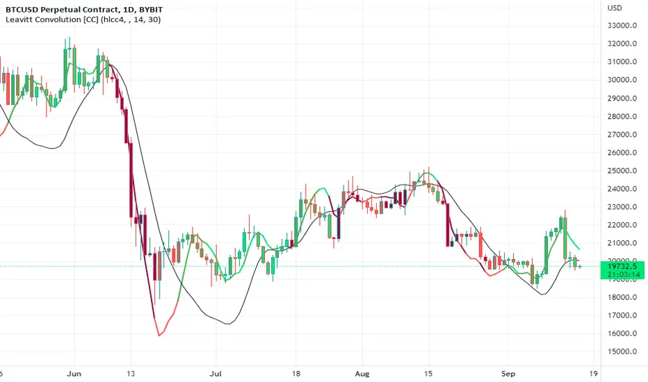
Leavitt Convolution [CC]The Leavitt Convolution indicator was created by Jay Leavitt (Stocks and Commodities Oct 2019, page 11), who is most well known for creating the Volume-Weighted Average Price indicator. This indicator is very similar to my Leavitt Projection script and I forgot to mention that both of these indicators are actually predictive moving averages. The Leavitt Convolution indicator doubles down on this idea by creating a prediction of the Leavitt Projection which is another prediction for the next bar. Obviously this means that it isn't always correct in its predictions but it does a very good job at predicting big trend changes before they happen. The recommended strategy for how to trade with these indicators is to plot a fast version and a slow version and go long when the fast version crosses over the slow version or to go short when the fast version crosses under the slow version. I have color coded the lines to turn light green for a normal buy signal or dark green for a strong buy signal and light red for a normal sell signal, and dark red for a strong sell signal.
This is another indicator in a series that I'm publishing to fulfill a special request from @ashok1961 so let me know if you ever have any special requests for me.
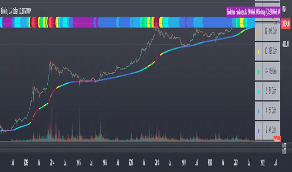
Blockchain Fundamentals: 200 Week MA Heatmap [CR]Blockchain Fundamentals: 200 Week MA Heatmap
This is released as a thank you to all my followers who pushed me over the 600 follower mark on twitter. Thanks to all you Kingz and Queenz out there who made it happen. <3
Indicator Overview
In each of its major market cycles, Bitcoin's price historically bottoms out around the 200 week moving average.
This indicator uses a color heatmap based on the % increases of that 200 week moving average. Depending on the rolling cumulative 4 week percent delta of the 200 week moving average, a color is assigned to the price chart. This method clearly highlights the market cycles of bitcoin and can be extremely helpful to use in your forecasts.
How It Can Be Used
The long term Bitcoin investor can monitor the monthly color changes. Historically, when we see orange and red dots assigned to the price chart, this has been a good time to sell Bitcoin as the market overheats. Periods where the price dots are purple and close to the 200 week MA have historically been good times to buy.
Bitcoin Price Prediction Using This Tool
If you are looking to predict the price of Bitcoin or forecast where it may go in the future, the 200WMA heatmap can be a useful tool as it shows on a historical basis whether the current price is overextending (red dots) and may need to cool down. It can also show when Bitcoin price may be good value on a historical basis. This can be when the dots on the chart are purple or blue.
Over more than ten years, $BTC has spent very little time below the 200 week moving average which is also worth noting when thinking about price predictions for Bitcoin or a Bitcoin price forecast.
Notes
1.) If you do not want to view the legend do the following: Indicator options > Style tab > Uncheck "Tables"
2.) I use my custom function to get around the limited historical data for bitcoin. You can check out the explanation of it here:
Nearest Neighbor Extrapolation of Price [Loxx]I wasn't going to post this because I don't like how this calculates by puling in the Open price, but I'm posting it anyway. This does work in it's current form but there is a. better way to do this. I'll revisit this in the future.
Anyway...
The k-Nearest Neighbor algorithm (k-NN) searches for k past patterns (neighbors) that are most similar to the current pattern and computes the future prices based on weighted voting of those neighbors. This indicator finds only one nearest neighbor. So, in essence, it is a 1-NN algorithm. It uses the Pearson correlation coefficient between the current pattern and all past patterns as the measure of distance between them. Also, this version of the nearest neighbor indicator gives larger weights to most recent prices while searching for the closest pattern in the past. It uses a weighted correlation coefficient, whose weight decays linearly from newer to older prices within a price pattern.
This indicator also includes an error window that shows whether the calculation is valid. If it's green and says "Passed", then the calculation is valid, otherwise it'll show a red background and and error message.
Inputs
Npast - number of past bars in a pattern;
Nfut -number of future bars in a pattern (must be < Npast).
lastbar - How many bars back to start forecast? Useful to show past prediction accuracy
barsbark - This prevents Pine from trying to calculate on all past bars
Related indicators
Hodrick-Prescott Extrapolation of Price
Itakura-Saito Autoregressive Extrapolation of Price
Helme-Nikias Weighted Burg AR-SE Extra. of Price
Weighted Burg AR Spectral Estimate Extrapolation of Price
Levinson-Durbin Autocorrelation Extrapolation of Price
Fourier Extrapolator of Price w/ Projection Forecast

Hodrick-Prescott Extrapolation of Price [Loxx]Hodrick-Prescott Extrapolation of Price is a Hodrick-Prescott filter used to extrapolate price.
The distinctive feature of the Hodrick-Prescott filter is that it does not delay. It is calculated by minimizing the objective function.
F = Sum((y(i) - x(i))^2,i=0..n-1) + lambda*Sum((y(i+1)+y(i-1)-2*y(i))^2,i=1..n-2)
where x() - prices, y() - filter values.
If the Hodrick-Prescott filter sees the future, then what future values does it suggest? To answer this question, we should find the digital low-frequency filter with the frequency parameter similar to the Hodrick-Prescott filter's one but with the values calculated directly using the past values of the "twin filter" itself, i.e.
y(i) = Sum(a(k)*x(i-k),k=0..nx-1) - FIR filter
or
y(i) = Sum(a(k)*x(i-k),k=0..nx-1) + Sum(b(k)*y(i-k),k=1..ny) - IIR filter
It is better to select the "twin filter" having the frequency-independent delay Тdel (constant group delay). IIR filters are not suitable. For FIR filters, the condition for a frequency-independent delay is as follows:
a(i) = +/-a(nx-1-i), i = 0..nx-1
The simplest FIR filter with constant delay is Simple Moving Average (SMA):
y(i) = Sum(x(i-k),k=0..nx-1)/nx
In case nx is an odd number, Тdel = (nx-1)/2. If we shift the values of SMA filter to the past by the amount of bars equal to Тdel, SMA values coincide with the Hodrick-Prescott filter ones. The exact math cannot be achieved due to the significant differences in the frequency parameters of the two filters.
To achieve the closest match between the filter values, I recommend their channel widths to be similar (for example, -6dB). The Hodrick-Prescott filter's channel width of -6dB is calculated as follows:
wc = 2*arcsin(0.5/lambda^0.25).
The channel width of -6dB for the SMA filter is calculated by numerical computing via the following equation:
|H(w)| = sin(nx*wc/2)/sin(wc/2)/nx = 0.5
Prediction algorithms:
The indicator features the two prediction methods:
Metod 1:
1. Set SMA length to 3 and shift it to the past by 1 bar. With such a length, the shifted SMA does not exist only for the last bar (Bar = 0), since it needs the value of the next future price Close(-1).
2. Calculate SMA filer's channel width. Equal it to the Hodrick-Prescott filter's one. Find lambda.
3. Calculate Hodrick-Prescott filter value at the last bar HP(0) and assume that SMA(0) with unknown Close(-1) gives the same value.
4. Find Close(-1) = 3*HP(0) - Close(0) - Close(1)
5. Increase the length of SMA to 5. Repeat all calculations and find Close(-2) = 5*HP(0) - Close(-1) - Close(0) - Close(1) - Close(2). Continue till the specified amount of future FutBars prices is calculated.
Method 2:
1. Set SMA length equal to 2*FutBars+1 and shift SMA to the past by FutBars
2. Calculate SMA filer's channel width. Equal it to the Hodrick-Prescott filter's one. Find lambda.
3. Calculate Hodrick-Prescott filter values at the last FutBars and assume that SMA behaves similarly when new prices appear.
4. Find Close(-1) = (2*FutBars+1)*HP(FutBars-1) - Sum(Close(i),i=0..2*FutBars-1), Close(-2) = (2*FutBars+1)*HP(FutBars-2) - Sum(Close(i),i=-1..2*FutBars-2), etc.
The indicator features the following inputs:
Method - prediction method
Last Bar - number of the last bar to check predictions on the existing prices (LastBar >= 0)
Past Bars - amount of previous bars the Hodrick-Prescott filter is calculated for (the more, the better, or at least PastBars>2*FutBars)
Future Bars - amount of predicted future values
The second method is more accurate but often has large spikes of the first predicted price. For our purposes here, this price has been filtered from being displayed in the chart. This is why method two starts its prediction 2 bars later than method 1. The described prediction method can be improved by searching for the FIR filter with the frequency parameter closer to the Hodrick-Prescott filter. For example, you may try Hanning, Blackman, Kaiser, and other filters with constant delay instead of SMA.
Related indicators
Itakura-Saito Autoregressive Extrapolation of Price
Helme-Nikias Weighted Burg AR-SE Extra. of Price
Weighted Burg AR Spectral Estimate Extrapolation of Price
Levinson-Durbin Autocorrelation Extrapolation of Price
Fourier Extrapolator of Price w/ Projection Forecast

Itakura-Saito Autoregressive Extrapolation of Price [Loxx]Itakura-Saito Autoregressive Extrapolation of Price is an indicator that uses an autoregressive analysis to predict future prices. This is a linear technique that was originally derived or speech analysis algorithms.
What is Itakura-Saito Autoregressive Analysis?
The technique of linear prediction has been available for speech analysis since the late 1960s (Itakura & Saito, 1973a, 1970; Atal & Hanauer, 1971), although the basic principles were established long before this by Wiener (1947). Linear predictive coding, which is also known as autoregressive analysis, is a time-series algorithm that has applications in many fields other than speech analysis (see, e.g., Chatfield, 1989).
Itakura and Saito developed a formulation for linear prediction analysis using a lattice form for the inverse filter. The Itakura–Saito distance (or Itakura–Saito divergence) is a measure of the difference between an original spectrum and an approximation of that spectrum. Although it is not a perceptual measure it is intended to reflect perceptual (dis)similarity. It was proposed by Fumitada Itakura and Shuzo Saito in the 1960s while they were with NTT. The distance is defined as: The Itakura–Saito distance is a Bregman divergence, but is not a true metric since it is not symmetric and it does not fulfil triangle inequality.
read more: Selected Methods for Improving Synthesis Speech Quality Using Linear Predictive Coding: System Description, Coefficient Smoothing and Streak
Data inputs
Source Settings: -Loxx's Expanded Source Types. You typically use "open" since open has already closed on the current active bar
LastBar - bar where to start the prediction
PastBars - how many bars back to model
LPOrder - order of linear prediction model; 0 to 1
FutBars - how many bars you want to forward predict
Things to know
Normally, a simple moving average is calculated on source data. I've expanded this to 38 different averaging methods using Loxx's Moving Avreages.
This indicator repaints
Related Indicators (linear extrapolation of price)
Levinson-Durbin Autocorrelation Extrapolation of Price
Weighted Burg AR Spectral Estimate Extrapolation of Price
Helme-Nikias Weighted Burg AR-SE Extra. of Price
Helme-Nikias Weighted Burg AR-SE Extra. of Price [Loxx]Helme-Nikias Weighted Burg AR-SE Extra. of Price is an indicator that uses an autoregressive spectral estimation called the Weighted Burg Algorithm, but unlike the usual WB algo, this one uses Helme-Nikias weighting. This method is commonly used in speech modeling and speech prediction engines. This is a linear method of forecasting data. You'll notice that this method uses a different weighting calculation vs Weighted Burg method. This new weighting is the following:
w = math.pow(array.get(x, i - 1), 2), the squared lag of the source parameter
and
w += math.pow(array.get(x, i), 2), the sum of the squared source parameter
This take place of the rectangular, hamming and parabolic weighting used in the Weighted Burg method
Also, this method includes Levinson–Durbin algorithm. as was already discussed previously in the following indicator:
Levinson-Durbin Autocorrelation Extrapolation of Price
What is Helme-Nikias Weighted Burg Autoregressive Spectral Estimate Extrapolation of price?
In this paper a new stable modification of the weighted Burg technique for autoregressive (AR) spectral estimation is introduced based on data-adaptive weights that are proportional to the common power of the forward and backward AR process realizations. It is shown that AR spectra of short length sinusoidal signals generated by the new approach do not exhibit phase dependence or line-splitting. Further, it is demonstrated that improvements in resolution may be so obtained relative to other weighted Burg algorithms. The method suggested here is shown to resolve two closely-spaced peaks of dynamic range 24 dB whereas the modified Burg schemes employing rectangular, Hamming or "optimum" parabolic windows fail.
Data inputs
Source Settings: -Loxx's Expanded Source Types. You typically use "open" since open has already closed on the current active bar
LastBar - bar where to start the prediction
PastBars - how many bars back to model
LPOrder - order of linear prediction model; 0 to 1
FutBars - how many bars you want to forward predict
Things to know
Normally, a simple moving average is calculated on source data. I've expanded this to 38 different averaging methods using Loxx's Moving Avreages.
This indicator repaints
Further reading
A high-resolution modified Burg algorithm for spectral estimation
Related Indicators
Levinson-Durbin Autocorrelation Extrapolation of Price
Weighted Burg AR Spectral Estimate Extrapolation of Price
Weighted Burg AR Spectral Estimate Extrapolation of Price [Loxx]Weighted Burg AR Spectral Estimate Extrapolation of Price is an indicator that uses an autoregressive spectral estimation called the Weighted Burg Algorithm. This method is commonly used in speech modeling and speech prediction engines. This method also includes Levinson–Durbin algorithm. As was already discussed previously in the following indicator:
Levinson-Durbin Autocorrelation Extrapolation of Price
What is Levinson recursion or Levinson–Durbin recursion?
In many applications, the duration of an uninterrupted measurement of a time series is limited. However, it is often possible to obtain several separate segments of data. The estimation of an autoregressive model from this type of data is discussed. A straightforward approach is to take the average of models estimated from each segment separately. In this way, the variance of the estimated parameters is reduced. However, averaging does not reduce the bias in the estimate. With the Burg algorithm for segments, both the variance and the bias in the estimated parameters are reduced by fitting a single model to all segments simultaneously. As a result, the model estimated with the Burg algorithm for segments is more accurate than models obtained with averaging. The new weighted Burg algorithm for segments allows combining segments of different amplitudes.
The Burg algorithm estimates the AR parameters by determining reflection coefficients that minimize the sum of for-ward and backward residuals. The extension of the algorithm to segments is that the reflection coefficients are estimated by minimizing the sum of forward and backward residuals of all segments taken together. This means a single model is fitted to all segments in one time. This concept is also used for prediction error methods in system identification, where the input to the system is known, like in ARX modeling
Data inputs
Source Settings: -Loxx's Expanded Source Types. You typically use "open" since open has already closed on the current active bar
LastBar - bar where to start the prediction
PastBars - how many bars back to model
LPOrder - order of linear prediction model; 0 to 1
FutBars - how many bars you want to forward predict
BurgWin - weighing function index, rectangular, hamming, or parabolic
Things to know
Normally, a simple moving average is calculated on source data. I've expanded this to 38 different averaging methods using Loxx's Moving Avreages.
This indicator repaints
Included
Bar color muting
Further reading
Performance of the weighted burg methods of ar spectral estimation for pitch-synchronous analysis of voiced speech
The Burg algorithm for segments
Techniques for the Enhancement of Linear Predictive Speech Coding in Adverse Conditions
Related Indicators

Levinson-Durbin Autocorrelation Extrapolation of Price [Loxx]Levinson-Durbin Autocorrelation Extrapolation of Price is an indicator that uses the Levinson recursion or Levinson–Durbin recursion algorithm to predict price moves. This method is commonly used in speech modeling and prediction engines.
What is Levinson recursion or Levinson–Durbin recursion?
Is a linear algebra prediction analysis that is performed once per bar using the autocorrelation method with a within a specified asymmetric window. The autocorrelation coefficients of the window are computed and converted to LP coefficients using the Levinson algorithm. The LP coefficients are then transformed to line spectrum pairs for quantization and interpolation. The interpolated quantized and unquantized filters are converted back to the LP filter coefficients to construct the synthesis and weighting filters for each bar.
Data inputs
Source Settings: -Loxx's Expanded Source Types. You typically use "open" since open has already closed on the current active bar
LastBar - bar where to start the prediction
PastBars - how many bars back to model
LPOrder - order of linear prediction model; 0 to 1
FutBars - how many bars you want to forward predict
Things to know
Normally, a simple moving average is caculated on source data. I've expanded this to 38 different averaging methods using Loxx's Moving Avreages.
This indicator repaints
Included
Bar color muting
Further reading
Implementing the Levinson-Durbin Algorithm on the StarCore™ SC140/SC1400 Cores
LevinsonDurbin_G729 Algorithm, Calculates LP coefficients from the autocorrelation coefficients. Intel® Integrated Performance Primitives for Intel® Architecture Reference Manual

Fourier Extrapolation of Variety Moving Averages [Loxx]Fourier Extrapolation of Variety Moving Averages is a Fourier Extrapolation (forecasting) indicator that has for inputs 38 different types of moving averages along with 33 different types of sources for those moving averages. This is a forecasting indicator of the selected moving average of the selected price of the underlying ticker. This indicator will repaint, so past signals are only as valid as the current bar. This indicator allows for up to 1500 bars between past bars and future projection bars. If the indicator won't load on your chart. check the error message for details on how to fix that, but you must ensure that past bars + futures bars is equal to or less than 1500.
Fourier Extrapolation using the Quinn-Fernandes algorithm is one of several (5-10) methods of signals forecasting that I'l be demonstrating in Pine Script.
What is Fourier Extrapolation?
This indicator uses a multi-harmonic (or multi-tone) trigonometric model of a price series xi, i=1..n, is given by:
xi = m + Sum( a*Cos(w*i) + b*Sin(w*i), h=1..H )
Where:
xi - past price at i-th bar, total n past prices;
m - bias;
a and b - scaling coefficients of harmonics;
w - frequency of a harmonic ;
h - harmonic number;
H - total number of fitted harmonics.
Fitting this model means finding m, a, b, and w that make the modeled values to be close to real values. Finding the harmonic frequencies w is the most difficult part of fitting a trigonometric model. In the case of a Fourier series, these frequencies are set at 2*pi*h/n. But, the Fourier series extrapolation means simply repeating the n past prices into the future.
This indicator uses the Quinn-Fernandes algorithm to find the harmonic frequencies. It fits harmonics of the trigonometric series one by one until the specified total number of harmonics H is reached. After fitting a new harmonic , the coded algorithm computes the residue between the updated model and the real values and fits a new harmonic to the residue.
see here: A Fast Efficient Technique for the Estimation of Frequency , B. G. Quinn and J. M. Fernandes, Biometrika, Vol. 78, No. 3 (Sep., 1991), pp . 489-497 (9 pages) Published By: Oxford University Press
The indicator has the following input parameters:
src - input source
npast - number of past bars, to which trigonometric series is fitted;
Nfut - number of predicted future bars;
nharm - total number of harmonics in model;
frqtol - tolerance of frequency calculations.
Included:
Loxx's Expanded Source Types
Loxx's Moving Averages
Other indicators using this same method
Fourier Extrapolator of Variety RSI w/ Bollinger Bands
Fourier Extrapolator of Price w/ Projection Forecast
Fourier Extrapolator of Price
Loxx's Moving Averages: Detailed explanation of moving averages inside this indicator
Loxx's Expanded Source Types: Detailed explanation of source types used in this indicator
Reverse Stoch [BApig Gift] - on PanelMssive credit to Motgench, Balipour and Wugamlo for this script. This script is all of their good work.
It is basically just the non-on chart version which I've slightly tweaked off their script. This can be useful to reduce the clutter on the chart itself. Releasing it in the hope that it can be useful for the community
Enjoy!

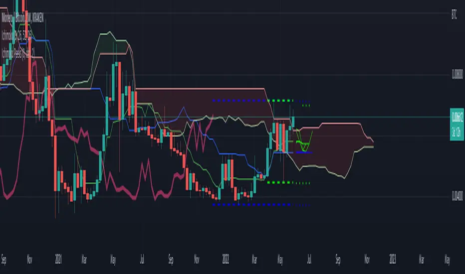
Ichimoku PeeksThis indicator uses the Ichimoku Tenkan / Kijun trend line formulas to predict what those values will be in the future if current price action does not violate the period highs and lows.
Because of the way Ichimoku formulates the trend, it contains (but does not visualize) this predictive information in a way that moving averages do not.
Sharp chart readers can infer upcoming changes by counting back candles, but the process can be automated, as I've shown here.
This description does not seem to be editable so implementation details and usage will be covered in code commentary.
Current bar predicted volumeDrag this indicator in the same panel with the volume in the object tree, then right click on the scale bar and set "merge all scale into one" for a correct visualization.
This indicator multiply the current traded volume of a candle with the total time of that candle. This offer a prediction of where, in case the volumes would keep trading at a comparable magnitude, the volume bar would close when the candle will close.
The predicted volume is indicated with a blue short line above the current volume bar, and updates in real time.
I find this indicator extremely useful to offer at a glance an idea of an ascending or descending volume pattern, that can serve as confirmation for a reversal or breakout for example.
Very suitable for short time frames, where decisions have to be taken fast.
Enjoy,
Luca.

BB Order BlocksUsing the Bollinger Band to mark areas of Support and Resistance
The scrip finds the highest and lowest levels of the bands to mark up futures areas of interest.
If the High/Lows are being broken on the Bollinger band, or if the look back range has expired without finding new levels, the script will stop plotting them until new levels are found
I have found many combinations which work well
Changing the band length to to levels 20,50,100 or 200 seem to give interesting results
Aswell as this changing the standard deviation to 3 instead of 2 marks up key levels.
The look back range seems to show better levels on 50,100 and 200
Let me know any changes or updates you think you could make an impact , this was just a quick basic script I wanted to share.

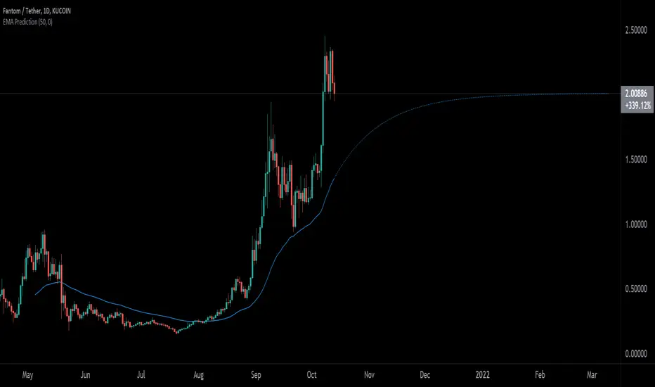
EMA PredictionThis script predicts future EMA values assuming that the price remains as configured (-50% to +50%).
Ehlers Optimum Predictor [CC]The Optimum Predictor was created by John Ehlers (Rocket Science For Traders pgs 209-210) and this indicator does a pretty good job of predicting major market moves. When the blue line crosses over the red line then this indicator is predicting an upcoming uptrend and when the blue line crosses under the red line then it is predicting an upcoming downtrend. Ehlers recommends using this indicator with an entire trading system to filter out any bad signals but most of the signals it gives are pretty accurate. He uses advanced digital signal processing to predict the future prices and uses it in an ema formula for the calculation. There are several ways to interpret this indicator: you can look for crossovers, you can also look for when the indicator goes above 0 for a general uptrend or below 0 for a general downtrend.
Let me know if there are any other scripts you would like to see me publish!

MACD Trendprediction Strategy V1A trend following indicator based on the MACD and EMA. In this case, signals are not generated by crossing the signal lines as with the MACD, but as soon as the distance between the signal lines increases or decreases. A profit factor of 1.6-3.5 is achieved.
Ein Trendfolge-Indikator, auf der Basis des MACD und EMA. Dabei werden Signale nicht wie bei dem MACD per Kreuzung der Signallinien generiert, sondern sobald ein der Abstand der Signallinien zu oder abnimmt.

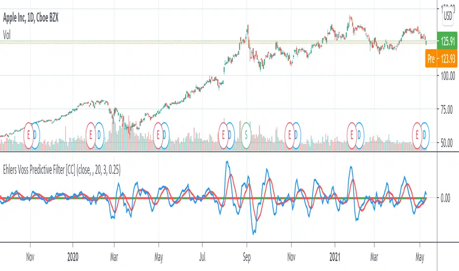
Ehlers Voss Predictive Filter [CC]The Voss Predictive Filter was created by John Ehlers (Stocks and Commodities August 2019) and this is a unique indicator in that it tries to predict future price action. I have color coded the middle line to show buy and sell signals so buy when the line turns green and sell when it turns red.
Let me know if there are any other indicators you want me to publish!
Multi Moving Average with ForecastThis script allows to use 5 different MAs with prediction of the next five periods.
Similarity Search, Karobein and Seasonal Random IndexSimilarity Search, Karobein oscillator (KO) and Seasonal Random Index (SRI)
Description:
This indicator uses dynamic capabilities of Pinescript version 4 coupled with Seasonal Random Index (SRI) and Karobein Oscillator (KO). SRI (green/red areas) is employed to detect trends and KO (black curce) is used to find historical similarities to predict the next bar's direction. The midline arrows are the predictions produced by the similarity search algorithm.
Machine Learning: kNN-based Strategy (update)kNN-based Strategy (FX and Crypto)
Description:
This update to the popular kNN-based strategy features:
improvements in the business logic,
an adjustible k value for the kNN model,
one more feature (MOM),
a streamlined signal filter and
some other minor fixes.
Now this script works in all timeframes !
I intentionally decided to publish this script separately
in order for the users to see the differences.
