Volume Weighted Average Price Dynamic Slope [sgbpulse]VWAP Dynamic Slope: A Comprehensive Indicator for Trend Identification and Smart Trading
Introducing VWAP Dynamic Slope, an innovative TradingView indicator that harnesses the power of Volume Weighted Average Price (VWAP) and enhances it with immediate visual feedback. The indicator colors the VWAP line based on its slope, allowing you to quickly and easily identify the direction and strength of the current trend for the asset, providing advanced tools for in-depth analysis.
What is VWAP and Why is it so Important?
VWAP (Volume Weighted Average Price) is an indicator that represents the average price at which an asset has traded, weighted by the volume traded at each price level. Unlike a simple moving average, VWAP gives greater weight to trades executed with high volume, making it a reliable measure of the asset's "true" or "fair" price within a given period. Many institutional traders use VWAP as a central reference point for evaluating the effectiveness of entries and exits. An asset trading above its VWAP is considered to have bullish momentum, and below it – bearish momentum.
How it Works: Dynamic VWAP Slope Analysis
VWAP Dynamic Slope analyzes the inclination of the VWAP line and displays it using an intuitive color scheme:
Positive Slope (Uptrend): When the VWAP points upwards, signaling positive momentum, the default color will be green.
Negative Slope (Downtrend): When the VWAP points downwards, signaling negative momentum, the default color will be orange.
Trend Change (CHG): When a change in the VWAP's trend direction occurs, a "CHG" label will be displayed. The label's color will be green if the change is to an uptrend, and orange if the change is to a downtrend.
Identifying Steep Slopes for Increased Momentum:
The indicator's uniqueness lies in its ability to identify "steep" slopes – rapid and particularly strong changes in the VWAP's direction. This indicates exceptionally strong momentum:
Steep Positive Slope: The VWAP color will change to dark green, indicating significant buying pressure.
Steep Negative Slope: The VWAP color will change to dark red, indicating significant selling pressure.
Dynamic Momentum Strength Label: In situations of steep slope (positive or negative), a dynamic label will be displayed with the change value of the VWAP at that point. This label allows you to monitor momentum strength, intensification, or weakening in real-time.
Advanced Analytical Tools for Complete Control
VWAP Dynamic Slope provides you with unprecedented flexibility through a variety of customizable tools:
Multiple VWAP Anchors and Visual Marking:
Common Time Anchors: Choose whether the VWAP resets at the beginning of each Session (daily), Week, Month, Quarter, Year, Decade, or Century.
Advanced Intraday Anchors: Within the Session, you can choose to calculate VWAP specifically for Pre-Market, Regular Hours, and Post-Market hours. This option is particularly crucial for intraday traders.
Important Event Anchors: The indicator allows for VWAP resets at significant milestones such as Earnings, Dividends, and Splits, for analyzing the market's immediate reaction.
Visual Anchor Marking: To enhance clarity and orientation, a Label ⚓ can be displayed at each selected anchor point, helping to immediately identify the start point of the VWAP calculation in the chosen context.
Customizable Bands (Up to Three on Each Side):
Add up to three Bands above and below the VWAP to identify areas of deviation and excursion from the average price. You have two calculation options:
Standard Deviation: Based on volatility and statistical distance from the VWAP.
Percentage: Defines fixed percentage-based bands from the VWAP.
Key Pre-Market Levels (Pre-Market High/Low):
Display the Pre-Market High and Low levels as separate lines on the chart. These lines often serve as important psychological support and resistance zones, allowing you to see how the VWAP behaves near them.
Full Customization and Precise Control:
VWAP Source Selection: Determine which price data type will be used for the VWAP calculation. The default is HLC3 (average of High, Low, and Close), but any other relevant data source available in TradingView can be selected.
Offset: Set an offset for the VWAP line, allowing you to shift it left or right on the time axis by a chosen number of bars.
Customizable Colors: Choose your preferred colors for each slope state, Pre-Market High/Low lines, and Bands.
Setting the "Steepness" Threshold (Per-mille Price Change Per Minute ‱/min with Auto-Adjustment): Determine the sensitivity for identifying a steep slope by setting the required change threshold in VWAP in terms of per-mille price change per minute (‱/min). The indicator performs smart adjustment for any timeframe you select on the chart (e.g., 30 seconds, 1 minute, 5 minutes, 10 minutes, etc.), ensuring that the "steepness" setting maintains consistency and relevance.
Examples for Setting the Steepness Threshold:
Suppose you set the steepness threshold to 0.3‱/min (per-mille price change per minute).
On a 30-second chart: The indicator will check if the VWAP changed by 0.15 ‱/min (half of the per-minute threshold) within a single bar. If so, the slope will be considered steep. Explanation: Since 30 seconds is half a minute, the indicator looks for a change that is half of the threshold set for a full minute.
On a 1-minute chart: The indicator will check if the VWAP changed by 0.3 ‱/min (the full per-minute threshold) within a single bar. If so, the slope will be considered steep. Explanation: Here, the bar represents a full minute, so we check the full threshold.
On a 5-minute chart: The indicator will check if the VWAP changed by 1.5 ‱/min (5 times the per-minute threshold) within a single bar. If so, the slope will be considered steep. Explanation: A 5-minute bar contains 5 minutes, so the cumulative change in VWAP needs to be 5 times greater to be considered "steep" on the same scale.
In summary, this setting allows you to precisely and uniformly control the sensitivity of steep slope detection across all timeframes, providing immense flexibility in analyzing the asset's momentum.
Advantages of Using Per-mille Price Change Per Minute (‱/min)
Using per-mille price change per minute (‱/min) offers several key advantages for your indicator:
Normalized and Objective Measurement: It provides a uniform scale for the VWAP's rate of change, regardless of the asset's price or nominal value. A 0.1 per-mille change per minute always carries the same relative significance.
Comparison Across Different Asset Prices: Using per-mille allows for direct comparison of VWAP movement strength between assets trading at very different prices (e.g., a $100 asset versus a $1 asset), enabling an understanding of true momentum without bias from the nominal price.
Smart Timeframe Agnostic Adjustment: This is a critical capability. The indicator automatically adjusts the per-mille per minute threshold you set to any chart timeframe (30 seconds, 1 minute, 5 minutes, etc.), maintaining consistency in "steepness" detection without manual recalibration.
Precise Momentum Identification: This measurement precisely identifies when the VWAP's rate of change becomes significant, and when momentum strengthens or weakens, contributing to more informed trading decisions.
In short, per-mille change per minute (‱/min) provides accuracy, consistency, and flexibility in identifying VWAP momentum changes, with smart adaptation across all timeframes.
Who is this Indicator For?
VWAP Dynamic Slope is a powerful tool for:
Intraday Traders: For quick identification of intraday trend directions and momentum across any timeframe, with specific consideration for Pre-Market, Regular Hours, or Post-Market VWAP, and incorporating key pre-market levels.
Swing Traders and Long-Term Investors: For analyzing longer-term trends based on periodic and event-driven VWAP anchors.
Beginner Traders: As an excellent visual aid for understanding the relationship between price, volume, and trend direction, and how different anchor points, pre-market levels, and data sources influence price behavior.
Experienced Traders: For integration with existing strategies, gaining additional confirmation for trend strength identification, and highly precise and flexible parameter calibration.
VWAP Dynamic Slope provides a rich, multi-dimensional layer of information about the VWAP, helping you make more informed trading decisions in real-time, within the context of your chosen asset.
Slope

TrendLibrary "Trend"
calculateSlopeTrend(source, length, thresholdMultiplier)
Parameters:
source (float)
length (int)
thresholdMultiplier (float)
Purpose:
The primary goal of this function is to determine the short-term trend direction of a given data series (like closing prices). It does this by calculating the slope of the data over a specified period and then comparing that slope against a dynamic threshold based on the data's recent volatility. It classifies the trend into one of three states: Upward, Downward, or Flat.
Parameters:
`source` (Type: `series float`): This is the input data series you want to analyze. It expects a series of floating-point numbers, typically price data like `close`, `open`, `hl2` (high+low)/2, etc.
`length` (Type: `int`): This integer defines the lookback period. The function will analyze the `source` data over the last `length` bars to calculate the slope and standard deviation.
`thresholdMultiplier` (Type: `float`, Default: `0.1`): This is a sensitivity factor. It's multiplied by the standard deviation to determine how steep the slope needs to be before it's considered a true upward or downward trend. A smaller value makes it more sensitive (detects trends earlier, potentially more false signals), while a larger value makes it less sensitive (requires a stronger move to confirm a trend).
Calculation Steps:
Linear Regression: It first calculates the value of a linear regression line fitted to the `source` data over the specified `length` (`ta.linreg(source, length, 0)`). Linear regression finds the "best fit" straight line through the data points.
Slope Calculation: It then determines the slope of this linear regression line. Since `ta.linreg` gives the *value* of the line on the current bar, the slope is calculated as the difference between the current bar's linear regression value (`linRegValue`) and the previous bar's value (`linRegValue `). A positive difference means an upward slope, negative means downward.
Volatility Measurement: It calculates the standard deviation (`ta.stdev(source, length)`) of the `source` data over the same `length`. Standard deviation is a measure of how spread out the data is, essentially quantifying its recent volatility.
Adaptive Threshold: An adaptive threshold (`threshold`) is calculated by multiplying the standard deviation (`stdDev`) by the `thresholdMultiplier`. This is crucial because it means the definition of a "flat" trend adapts to the market's volatility. In volatile times, the threshold will be wider, requiring a larger slope to signal a trend. In quiet times, the threshold will be narrower.
Trend Determination: Finally, it compares the calculated `slope` to the adaptive `threshold`:
If the `slope` is greater than the positive `threshold`, the trend is considered **Upward**, and the function returns `1`.
If the `slope` is less than the negative `threshold` (`-threshold`), the trend is considered **Downward**, and the function returns `-1`.
If the `slope` falls between `-threshold` and `+threshold` (inclusive of 0), the trend is considered **Flat**, and the function returns `0`.
Return Value:
The function returns an integer representing the determined trend direction:
`1`: Upward trend
`-1`: Downward trend
`0`: Flat trend
In essence, this library function provides a way to gauge trend direction using linear regression, but with a smart filter (the adaptive threshold) to avoid classifying minor noise or low-volatility periods as significant trends.
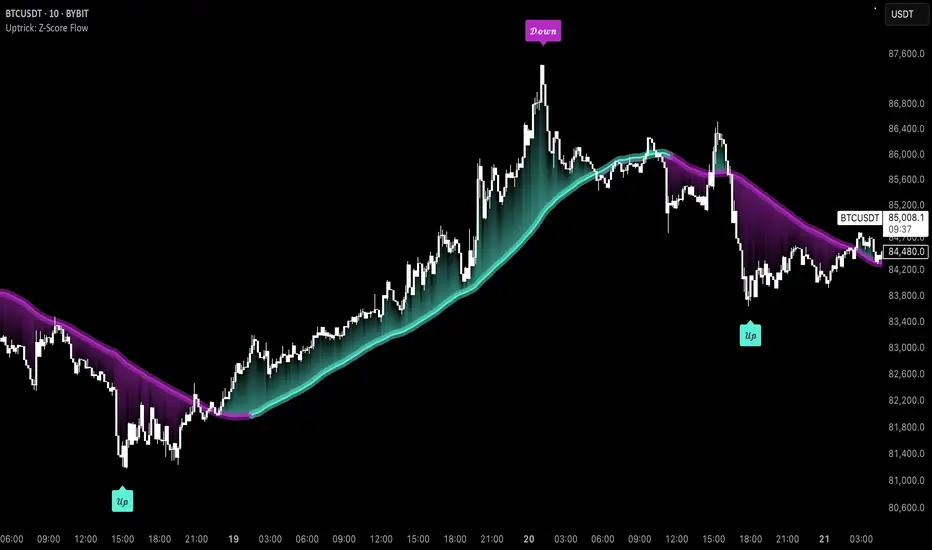
Uptrick: Z-Score FlowOverview
Uptrick: Z-Score Flow is a technical indicator that integrates trend-sensitive momentum analysi s with mean-reversion logic derived from Z-Score calculations. Its primary objective is to identify market conditions where price has either stretched too far from its mean (overbought or oversold) or sits at a statistically “normal” range, and then cross-reference this observation with trend direction and RSI-based momentum signals. The result is a more contextual approach to trade entry and exit, emphasizing precision, clarity, and adaptability across varying market regimes.
Introduction
Financial instruments frequently transition between trending modes, where price extends strongly in one direction, and ranging modes, where price oscillates around a central value. A simple statistical measure like Z-Score can highlight price extremes by comparing the current price against its historical mean and standard deviation. However, such extremes alone can be misleading if the broader market structure is trending forcefully. Uptrick: Z-Score Flow aims to solve this gap by combining Z-Score with an exponential moving average (EMA) trend filter and a smoothed RSI momentum check, thus filtering out signals that contradict the prevailing market environment.
Purpose
The purpose of this script is to help traders pinpoint both mean-reversion opportunities and trend-based pullbacks in a way that is statistically grounded yet still mindful of overarching price action. By pairing Z-Score thresholds with supportive conditions, the script reduces the likelihood of acting on random price spikes or dips and instead focuses on movements that are significant within both historical and current contextual frameworks.
Originality and Uniquness
Layered Signal Verification: Signals require the fulfillment of multiple layers (Z-Score extreme, EMA trend bias, and RSI momentum posture) rather than merely breaching a statistical threshold.
RSI Zone Lockout: Once RSI enters an overbought/oversold zone and triggers a signal, the script locks out subsequent signals until RSI recovers above or below those zones, limiting back-to-back triggers.
Controlled Cooldown: A dedicated cooldown mechanic ensures that the script waits a specified number of bars before issuing a new signal in the opposite direction.
Gradient-Based Visualization: Distinct gradient fills between price and the Z-Mean line enhance readability, showing at a glance whether price is trading above or below its statistical average.
Comprehensive Metrics Panel: An optional on-chart table summarizes the Z-Score’s key metrics, streamlining the process of verifying current statistical extremes, mean levels, and momentum directions.
Why these indicators were merged
Z-Score measurements excel at identifying when price deviates from its mean, but they do not intrinsically reveal whether the market’s trajectory supports a reversion or if price might continue along its trend. The EMA, commonly used for spotting trend directions, offers valuable insight into whether price is predominantly ascending or descending. However, relying solely on a trend filter overlooks the intensity of price moves. RSI then adds a dedicated measure of momentum, helping confirm if the market’s energy aligns with a potential reversal (for example, price is statistically low but RSI suggests looming upward momentum). By uniting these three lenses—Z-Score for statistical context, EMA for trend direction, and RSI for momentum force—the script offers a more comprehensive and adaptable system, aiming to avoid false positives caused by focusing on just one aspect of price behavior.
Calculations
The core calculation begins with a simple moving average (SMA) of price over zLen bars, referred to as the basis. Next, the script computes the standard deviation of price over the same window. Dividing the difference between the current price and the basis by this standard deviation produces the Z-Score, indicating how many standard deviations the price is from its mean. A positive Z-Score reveals price is above its average; a negative reading indicates the opposite.
To detect overall market direction, the script calculates an exponential moving average (emaTrend) over emaTrendLen bars. If price is above this EMA, the script deems the market bullish; if below, it’s considered bearish. For momentum confirmation, the script computes a standard RSI over rsiLen bars, then applies a smoothing EMA over rsiEmaLen bars. This smoothed RSI (rsiEma) is monitored for both its absolute level (oversold or overbought) and its slope (the difference between the current and previous value). Finally, slopeIndex determines how many bars back the script compares the basis to check whether the Z-Mean line is generally rising, falling, or flat, which then informs the coloring scheme on the chart.
Calculations and Rational
Simple Moving Average for Baseline: An SMA is used for the core mean because it places equal weight on each bar in the lookback period. This helps maintain a straightforward interpretation of overbought or oversold conditions in the context of a uniform historical average.
Standard Deviation for Volatility: Standard deviation measures the variability of the data around the mean. By dividing price’s difference from the mean by this value, the Z-Score can highlight whether price is unusually stretched given typical volatility.
Exponential Moving Average for Trend: Unlike an SMA, an EMA places more emphasis on recent data, reacting quicker to new price developments. This quicker response helps the script promptly identify trend shifts, which can be crucial for filtering out signals that go against a strong directional move.
RSI for Momentum Confirmation: RSI is an oscillator that gauges price movement strength by comparing average gains to average losses over a set period. By further smoothing this RSI with another EMA, short-lived oscillations become less influential, making signals more robust.
SlopeIndex for Slope-Based Coloring: To clarify whether the market’s central tendency is rising or falling, the script compares the basis now to its level slopeIndex bars ago. A higher current reading indicates an upward slope; a lower reading, a downward slope; and similar readings, a flat slope. This is visually represented on the chart, providing an immediate sense of the directionality.
Inputs
zLen (Z-Score Period)
Specifies how many bars to include for computing the SMA and standard deviation that form the basis of the Z-Score calculation. Larger values produce smoother but slower signals; smaller values catch quick changes but may generate noise.
emaTrendLen (EMA Trend Filter)
Sets the length of the EMA used to detect the market’s primary direction. This is pivotal for distinguishing whether signals should be considered (price aligning with an uptrend or downtrend) or filtered out.
rsiLen (RSI Length)
Defines the window for the initial RSI calculation. This RSI, when combined with the subsequent smoothing EMA, forms the foundation for momentum-based signal confirmations.
rsiEmaLen (EMA of RSI Period)
Applies an exponential moving average over the RSI readings for additional smoothing. This step helps mitigate rapid RSI fluctuations that might otherwise produce whipsaw signals.
zBuyLevel (Z-Score Buy Threshold)
Determines how negative the Z-Score must be for the script to consider a potential oversold signal. If the Z-Score dives below this threshold (and other criteria are met), a buy signal is generated.
zSellLevel (Z-Score Sell Threshold)
Determines how positive the Z-Score must be for a potential overbought signal. If the Z-Score surpasses this threshold (and other checks are satisfied), a sell signal is generated.
cooldownBars (Cooldown (Bars))
Enforces a bar-based delay between opposite signals. Once a buy signal has fired, the script must wait the specified number of bars before registering a new sell signal, and vice versa.
slopeIndex (Slope Sensitivity (Bars))
Specifies how many bars back the script compares the current basis for slope coloration. A bigger slopeIndex highlights larger directional trends, while a smaller number emphasizes shorter-term shifts.
showMeanLine (Show Z-Score Mean Line)
Enables or disables the plotting of the Z-Mean and its slope-based coloring. Traders who prefer minimal chart clutter may turn this off while still retaining signals.
Features
Statistical Core (Z-Score Detection):
This feature computes the Z-Score by taking the difference between the current price and the basis (SMA) and dividing by the standard deviation. In effect, it translates price fluctuations into a standardized measure that reveals how significant a move is relative to the typical variation seen over the lookback. When the Z-Score crosses predefined thresholds (zBuyLevel for oversold and zSellLevel for overbought), it signals that price could be at an extreme.
How It Works: On each bar, the script updates the SMA and standard deviation. The Z-Score is then refreshed accordingly. Traders can interpret particularly large negative or positive Z-Score values as scenarios where price is abnormally low or high.
EMA Trend Filter:
An EMA over emaTrendLen bars is used to classify the market as bullish if the price is above it and bearish if the price is below it. This classification is applied to the Z-Score signals, accepting them only when they align with the broader price direction.
How It Works: If the script detects a Z-Score below zBuyLevel, it further checks if price is actually in a downtrend (below EMA) before issuing a buy signal. This might seem counterintuitive, but a “downtrend” environment plus an oversold reading often signals a potential bounce or a mean-reversion play. Conversely, for sell signals, the script checks if the market is in an uptrend first. If it is, an overbought reading aligns with potential profit-taking.
RSI Momentum Confirmation with Oversold/Overbought Lockout:
RSI is calculated over rsiLen, then smoothed by an EMA over rsiEmaLen. If this smoothed RSI dips below a certain threshold (for example, 30) and then begins to slope upward, the indicator treats it as a potential sign of recovering momentum. Similarly, if RSI climbs above a certain threshold (for instance, 70) and starts to slope downward, that suggests dwindling momentum. Additionally, once RSI is in these zones, the indicator locks out repetitive signals until RSI fully exits and re-enters those extreme territories.
How It Works: Each bar, the script measures whether RSI has dropped below the oversold threshold (like 30) and has a positive slope. If it does, the buy side is considered “unlocked.” For sell signals, RSI must exceed an overbought threshold (70) and slope downward. The combination of threshold and slope helps confirm that a reversal is genuinely in progress instead of issuing signals while momentum remains weak or stuck in extremes.
Cooldown Mechanism:
The script features a custom bar-based cooldown that prevents issuing new signals in the opposite direction immediately after one is triggered. This helps avoid whipsaw situations where the market quickly flips from oversold to overbought or vice versa.
How It Works: When a buy signal fires, the indicator notes the bar index. If the Z-Score and RSI conditions later suggest a sell, the script compares the current bar index to the last buy signal’s bar index. If the difference is within cooldownBars, the signal is disallowed. This ensures a predefined “quiet period” before switching signals.
Slope-Based Coloring (Z-Mean Line and Shadow):
The script compares the current basis value to its value slopeIndex bars ago. A higher reading now indicates a generally upward slope, while a lower reading indicates a downward slope. The script then shades the Z-Mean line in a corresponding bullish or bearish color, or remains neutral if little change is detected.
How It Works: This slope calculation is refreshingly straightforward: basis – basis . If the result is positive, the line is colored bullish; if negative, it is colored bearish; if approximately zero, it remains neutral. This provides a quick visual cue of the medium-term directional bias.
Gradient Overlays:
With gradient fills, the script highlights where price stands in relation to the Z-Mean. When price is above the basis, a purple-shaded region is painted, visually indicating a “bearish zone” for potential overbought conditions. When price is below, a teal-like overlay is used, suggesting a “bullish zone” for potential oversold conditions.
How It Works: Each bar, the script checks if price is above or below the basis. It then applies a fill between close and basis, using distinct colors to show whether the market is trading above or below its mean. This creates an immediate sense of how extended the market might be.
Buy and Sell Labels (with Alerts):
When a legitimate buy or sell condition passes every check (Z-Score threshold, EMA trend alignment, RSI gating, and cooldown clearance), the script plots a corresponding label directly on the chart. It also fires an alert (if alerts are set up), making it convenient for traders who want timely notifications.
How It Works: If rawBuy or rawSell conditions are met (refined by RSI, EMA trend, and cooldown constraints), the script calls the respective plot function to paint an arrow label on the chart. Alerts are triggered simultaneously, carrying easily recognizable messages.
Metrics Table:
The optional on-chart table (activated by showMetrics) presents real-time Z-Score data, including the current Z-Score, its rolling mean, the maximum and minimum Z-Score values observed over the last zLen bars, a percentile position, and a short-term directional note (rising, falling, or flat).
Current – The present Z-Score reading
Mean – Average Z-Score over the zLen period
Min/Max – Lowest and highest Z-Score values within zLen
Position – Where the current Z-Score sits between the min and max (as a percentile)
Trend – Whether the Z-Score is increasing, decreasing, or flat
Conclusion
Uptrick: Z-Score Flow offers a versatile solution for traders who need a statistically informed perspective on price extremes combined with practical checks for overall trend and momentum. By leveraging a well-defined combination of Z-Score, EMA trend classification, RSI-based momentum gating, slope-based visualization, and a cooldown mechanic, the script reduces the occurrence of false or premature signals. Its gradient fills and optional metrics table contribute further clarity, ensuring that users can quickly assess market posture and make more confident trading decisions in real time.
Disclaimer
This script is intended solely for informational and educational purposes. Trading in any financial market comes with substantial risk, and there is no guarantee of success or the avoidance of loss. Historical performance does not ensure future results. Always conduct thorough research and consider professional guidance prior to making any investment or trading decisions.
Multi-Anchored Linear Regression Channels [TANHEF]█ Overview:
The 'Multi-Anchored Linear Regression Channels ' plots multiple dynamic regression channels (or bands) with unique selectable calculation types for both regression and deviation. It leverages a variety of techniques, customizable anchor sources to determine regression lengths, and user-defined criteria to highlight potential opportunities.
Before getting started, it's worth exploring all sections, but make sure to review the Setup & Configuration section in particular. It covers key parameters like anchor type, regression length, bias, and signal criteria—essential for aligning the tool with your trading strategy.
█ Key Features:
⯁ Multi-Regression Capability:
Plot up to three distinct regression channels and/or bands simultaneously, each with customizable anchor types to define their length.
⯁ Regression & Deviation Methods:
Regressions Types:
Standard: Uses ordinary least squares to compute a simple linear trend by averaging the data and deriving a slope and endpoints over the lookback period.
Ridge: Introduces L2 regularization to stabilize the slope by penalizing large coefficients, which helps mitigate multicollinearity in the data.
Lasso: Uses L1 regularization through soft-thresholding to shrink less important coefficients, yielding a simpler model that highlights key trends.
Elastic Net: Combines L1 and L2 penalties to balance coefficient shrinkage and selection, producing a robust weighted slope that handles redundant predictors.
Huber: Implements the Huber loss with iteratively reweighted least squares (IRLS) and EMA-style weights to reduce the impact of outliers while estimating the slope.
Least Absolute Deviations (LAD): Reduces absolute errors using iteratively reweighted least squares (IRLS), yielding a slope less sensitive to outliers than squared-error methods.
Bayesian Linear: Merges prior beliefs with weighted data through Bayesian updating, balancing the prior slope with data evidence to derive a probabilistic trend.
Deviation Types:
Regressive Linear (Reverse): In reverse order (recent to oldest), compute weighted squared differences between the data and a line defined by a starting value and slope.
Progressive Linear (Forward): In forward order (oldest to recent), compute weighted squared differences between the data and a line defined by a starting value and slope.
Balanced Linear: In forward order (oldest to newest), compute regression, then pair to source data in reverse order (newest to oldest) to compute weighted squared differences.
Mean Absolute: Compute weighted absolute differences between each data point and its regression line value, then aggregate them to yield an average deviation.
Median Absolute: Determine the weighted median of the absolute differences between each data point and its regression line value to capture the central tendency of deviations.
Percent: Compute deviation as a percentage of a base value by multiplying that base by the specified percentage, yielding symmetric positive and negative deviations.
Fitted: Compare a regression line with high and low series values by computing weighted differences to determine the maximum upward and downward deviations.
Average True Range: Iteratively compute the weighted average of absolute differences between the data and its regression line to yield an ATR-style deviation measure.
Bias:
Bias: Applies EMA or inverse-EMA style weighting to both Regression and/or Deviation, emphasizing either recent or older data.
⯁ Customizable Regression Length via Anchors:
Anchor Types:
Fixed: Length.
Bar-Based: Bar Highest/Lowest, Volume Highest/Lowest, Spread Highest/Lowest.
Correlation: R Zero, R Highest, R Lowest, R Absolute.
Slope: Slope Zero, Slope Highest, Slope Lowest, Slope Absolute.
Indicator-Based: Indicators Highest/Lowest (ADX, ATR, BBW, CCI, MACD, RSI, Stoch).
Time-Based: Time (Day, Week, Month, Quarter, Year, Decade, Custom).
Session-Based: Session (Tokyo, London, New York, Sydney, Custom).
Event-Based: Earnings, Dividends, Splits.
External: Input Source Highest/Lowest.
Length Selection:
Maximum: The highest allowed regression length (also fixed value of “Length” anchor).
Minimum: The shortest allowed length, ensuring enough bars for a valid regression.
Step: The sampling interval (e.g., 1 checks every bar, 2 checks every other bar, etc.). Increasing the step reduces the loading time, most applicable to “Slope” and “R” anchors.
Adaptive lookback:
Adaptive Lookback: Enable to display regression regardless of too few historical bars.
⯁ Selecting Bias:
Bias applies separately to regression and deviation.
Positive values emphasize recent data (EMA-style), negative invert, and near-zero maintains balance. (e.g., a length 100, bias +1 gives the newest price ~7× more weight than the oldest).
It's best to apply bias to both (regression and deviation) or just the deviation. Biasing only regression may distort deviation visually, while biasing both keeps their relationship intuitive. Using bias only for deviation scales it without altering regression, offering unique analysis.
⯁ Scale Awareness:
Supports linear and logarithmic price scaling, the regression and deviations adjust accordingly.
⯁ Signal Generation & Alerts:
Customizable entry/exit signals and alerts, detailed in the dedicated section below.
⯁ Visual Enhancements & Real-World Examples:
Optional on-chart table display summarizing regression input criteria (display type, anchor type, source, regression type, regression bias, deviation type, deviation bias, deviation multiplier) and key calculated metrics (regression length, slope, Pearson’s R, percentage position within deviations, etc.) for quick reference.
█ Understanding R (Pearson Correlation Coefficient):
Pearson’s R gauges data alignment to a straight-line trend within the regression length:
Range: R varies between –1 and +1.
R = +1 → Perfect positive correlation (strong uptrend).
R = 0 → No linear relationship detected.
R = –1 → Perfect negative correlation (strong downtrend).
This script uses Pearson’s R as an anchor, adjusting regression length to target specific R traits. Strong R (±1) follows the regression channel, while weak R (0) shows inconsistency.
█ Understanding the Slope:
The slope is the direction and rate at which the regression line rises or falls per bar:
Positive Slope (>0): Uptrend – Steeper means faster increase.
Negative Slope (<0): Downtrend – Steeper means sharper drop.
Zero or Near-Zero Slope: Sideways – Indicating range-bound conditions.
This script uses highest and lowest slope as an anchor, where extremes highlight strong moves and trend lines, while values near zero indicate sideways action and possible support/resistance.
█ Setup & Configuration:
Whether you’re new to this script or want to quickly adjust all critical parameters, the panel below shows the main settings available. You can customize everything from the anchor type and maximum length to the bias, signal conditions, and more.
Scale (select Log Scale for logarithmic, otherwise linear scale).
Display (regression channel and/or bands).
Anchor (how regression length is determined).
Length (control bars analyzed):
• Max – Upper limit.
• Min – Prevents regression from becoming too short.
• Step – Controls scanning precision; increasing Step reduces load time.
Regression:
• Type – Calculation method.
• Bias – EMA-style emphasis (>0=new bars weighted more; <0=old bars weighted more).
Deviation:
• Type – Calculation method.
• Bias – EMA-style emphasis (>0=new bars weighted more; <0=old bars weighted more).
• Multiplier - Adjusts Upper and Lower Deviation.
Signal Criteria:
• % (Price vs Deviation) – (0% = lower deviation, 50% = regression, 100% = upper deviation).
• R – (0 = no correlation, ±1 = perfect correlation; >0 = +slope, <0 = -slope).
Table (analyze table of input settings, calculated results, and signal criteria).
Adaptive Lookback (display regression while too few historical bars).
Multiple Regressions (steps 2 to 7 apply to #1, #2, and #3 regressions).
█ Signal Generation & Alerts:
The script offers customizable entry and exit signals with flexible criteria and visual cues (background color, dots, or triangles). Alerts can also be triggered for these opportunities.
Percent Direction Criteria:
(0% = lower deviation, 50% = regression line, 100% = upper deviation)
Above %: Triggers if price is above a specified percent of the deviation channel.
Below %: Triggers if price is below a specified percent of the deviation channel.
(Blank): Ignores the percent‐based condition.
Pearson's R (Correlation) Direction Criteria:
(0 = no correlation, ±1 = perfect correlation; >0 = positive slope, <0 = negative slope)
Above R / Below R: Compares the correlation to a threshold.
Above│R│ / Below│R│: Uses absolute correlation to focus on strength, ignoring direction.
Zero to R: Checks if R is in the 0-to-threshold range.
(Blank): Ignores correlation-based conditions.
█ User Tips & Best Practices:
Choose an anchor type that suits your strategy, “Bar Highest/Lowest” automatically spots commonly used regression zones, while “│R│ Highest” targets strong linear trends.
Consider enabling or disabling the Adaptive Lookback feature to ensure you always have a plotted regression if your chart doesn’t meet the maximum-length requirement.
Use a small Step size (1) unless relying on R-correlation or slope-based anchors as the are time-consuming to calculate. Larger steps speed up calculations but reduce precision.
Fine-tune settings such as lookback periods, regression bias, and deviation multipliers, or trend strength. Small adjustments can significantly affect how channels and signals behave.
To reduce loading time , show only channels (not bands) and disable signals, this limits calculations to the last bar and supports more extreme criteria.
Use the table display to monitor anchor type, calculated length, slope, R value, and percent location at a glance—especially if you have multiple regressions visible simultaneously.
█ Conclusion:
With its blend of advanced regression techniques, flexible deviation options, and a wide range of anchor types, this indicator offers a highly adaptable linear regression channeling system. Whether you're anchoring to time, price extremes, correlation, slope, or external events, the tool can be shaped to fit a variety of strategies. Combined with customizable signals and alerts, it may help highlight areas of confluence and support a more structured approach to identifying potential opportunities.

LinearRegressionLibrary "LinearRegression"
Calculates a variety of linear regression and deviation types, with optional emphasis weighting. Additionally, multiple of slope and Pearson’s R calculations.
calcSlope(_src, _len, _condition)
Calculates the slope of a linear regression over the specified length.
Parameters:
_src (float) : (float) The source data.
_len (int) : (int) The length of the lookback period for the linear regression.
_condition (bool) : (bool) Flag to enable calculation. Set to true to calculate on every bar; otherwise, set to barstate.islast for efficiency.
Returns: (float) The slope of the linear regression.
calcReg(_src, _len, _condition)
Calculates a basic linear regression, returning y1, y2, slope, and average.
Parameters:
_src (float) : (float) The source data series.
_len (int) : (int) The length of the lookback period.
_condition (bool) : (bool) Flag to enable calculation (true = calculate).
Returns: (float ) An array of 4 values: .
calcRegStandard(_src, _len, _emphasis, _condition)
Calculates an Standard linear regression with optional emphasis.
Parameters:
_src (float) : (series float) The source data series.
_len (int) : (int) The length of the lookback period.
_emphasis (float) : (float) The emphasis factor: 0 for equal weight; >0 emphasizes recent bars; <0 emphasizes older bars.
_condition (bool) : (bool) Flag to enable calculation (true = calculate).
Returns: (float ) .
calcRegRidge(_src, _len, lambda, _emphasis, _condition)
Calculates a ridge regression with optional emphasis.
Parameters:
_src (float) : (float) The source data series.
_len (int) : (int) The length of the lookback period.
lambda (float) : (float) The ridge regularization parameter.
_emphasis (float) : (float) The emphasis factor: 0 for equal weight; >0 emphasizes recent bars; <0 emphasizes older bars.
_condition (bool) : (bool) Flag to enable calculation (true = calculate).
Returns: (float ) .
calcRegLasso(_src, _len, lambda, _emphasis, _condition)
Calculates a Lasso regression with optional emphasis.
Parameters:
_src (float) : (float) The source data series.
_len (int) : (int) The length of the lookback period.
lambda (float) : (float) The Lasso regularization parameter.
_emphasis (float) : (float) The emphasis factor: 0 for equal weight; >0 emphasizes recent bars; <0 emphasizes older bars.
_condition (bool) : (bool) Flag to enable calculation (true = calculate).
Returns: (float ) .
calcElasticNetLinReg(_src, _len, lambda1, lambda2, _emphasis, _condition)
Calculates an Elastic Net regression with optional emphasis.
Parameters:
_src (float) : (float) The source data series.
_len (int) : (int) The length of the lookback period.
lambda1 (float) : (float) L1 regularization parameter (Lasso).
lambda2 (float) : (float) L2 regularization parameter (Ridge).
_emphasis (float) : (float) Emphasis factor: 0 for equal weight; >0 emphasizes recent bars; <0 emphasizes older bars.
_condition (bool) : (bool) Flag to enable calculation (true = calculate).
Returns: (float ) .
calcRegHuber(_src, _len, delta, iterations, _emphasis, _condition)
Calculates a Huber regression using Iteratively Reweighted Least Squares (IRLS).
Parameters:
_src (float) : (float) The source data series.
_len (int) : (int) The length of the lookback period.
delta (float) : (float) Huber threshold parameter.
iterations (int) : (int) Number of IRLS iterations.
_emphasis (float) : (float) Emphasis factor: 0 for equal weight; >0 emphasizes recent bars; <0 emphasizes older bars.
_condition (bool) : (bool) Flag to enable calculation (true = calculate).
Returns: (float ) .
calcRegLAD(_src, _len, iterations, _emphasis, _condition)
Calculates a Least Absolute Deviations (LAD) regression via IRLS.
Parameters:
_src (float) : (float) The source data series.
_len (int) : (int) The length of the lookback period.
iterations (int) : (int) Number of IRLS iterations for LAD.
_emphasis (float) : (float) Emphasis factor: 0 for equal weight; >0 emphasizes recent bars; <0 emphasizes older bars.
_condition (bool) : (bool) Flag to enable calculation (true = calculate).
Returns: (float ) .
calcRegBayesian(_src, _len, priorMean, priorSpan, sigma, _emphasis, _condition)
Calculates a Bayesian linear regression with optional emphasis.
Parameters:
_src (float) : (float) The source data series.
_len (int) : (int) The length of the lookback period.
priorMean (float) : (float) The prior mean for the slope.
priorSpan (float) : (float) The prior variance (or span) for the slope.
sigma (float) : (float) The assumed standard deviation of residuals.
_emphasis (float) : (float) Emphasis factor: 0 for equal weight; >0 emphasizes recent bars; <0 emphasizes older bars.
_condition (bool) : (bool) Flag to enable calculation (true = calculate).
Returns: (float ) .
calcRFromLinReg(_src, _len, _slope, _average, _y1, _condition)
Calculates the Pearson correlation coefficient (R) based on linear regression parameters.
Parameters:
_src (float) : (float) The source data.
_len (int) : (int) The length of the lookback period.
_slope (float) : (float) The slope of the linear regression.
_average (float) : (float) The average value of the source data series.
_y1 (float) : (float) The starting point (y-intercept of the oldest bar) for the linear regression.
_condition (bool) : (bool) Flag to enable calculation. Set to true to calculate on every bar; otherwise, set to barstate.islast for efficiency.
Returns: (float) The Pearson correlation coefficient (R) adjusted for the direction of the slope.
calcRFromSource(_src, _len, _condition)
Calculates the correlation coefficient (R) using a specified length and source data.
Parameters:
_src (float) : (float) The source data.
_len (int) : (int) The length of the lookback period.
_condition (bool) : (bool) Flag to enable calculation. Set to true to calculate on every bar; otherwise, set to barstate.islast for efficiency.
Returns: (float) The correlation coefficient (R).
calcSlopeLengthZero(_src, _len, _minLen, _step, _condition)
Identifies the length at which the slope is flattest (closest to zero).
Parameters:
_src (float) : (float) The source data.
_len (int) : (int) The maximum lookback length to consider (minimum of 2).
_minLen (int) : (int) The minimum length to start from (cannot exceed the max length).
_step (int) : (int) The increment step for lengths.
_condition (bool) : (bool) Flag to enable calculation. Set to true to calculate on every bar; otherwise, set to barstate.islast.
Returns: (int) The length at which the slope is flattest.
calcSlopeLengthHighest(_src, _len, _minLen, _step, _condition)
Identifies the length at which the slope is highest.
Parameters:
_src (float) : (float) The source data.
_len (int) : (int) The maximum lookback length (minimum of 2).
_minLen (int) : (int) The minimum length to start from.
_step (int) : (int) The step for incrementing lengths.
_condition (bool) : (bool) Flag to enable calculation. Set to true to calculate on every bar; otherwise, set to barstate.islast.
Returns: (int) The length at which the slope is highest.
calcSlopeLengthLowest(_src, _len, _minLen, _step, _condition)
Identifies the length at which the slope is lowest.
Parameters:
_src (float) : (float) The source data.
_len (int) : (int) The maximum lookback length (minimum of 2).
_minLen (int) : (int) The minimum length to start from.
_step (int) : (int) The step for incrementing lengths.
_condition (bool) : (bool) Flag to enable calculation. Set to true to calculate on every bar; otherwise, set to barstate.islast.
Returns: (int) The length at which the slope is lowest.
calcSlopeLengthAbsolute(_src, _len, _minLen, _step, _condition)
Identifies the length at which the absolute slope value is highest.
Parameters:
_src (float) : (float) The source data.
_len (int) : (int) The maximum lookback length (minimum of 2).
_minLen (int) : (int) The minimum length to start from.
_step (int) : (int) The step for incrementing lengths.
_condition (bool) : (bool) Flag to enable calculation. Set to true to calculate on every bar; otherwise, set to barstate.islast.
Returns: (int) The length at which the absolute slope value is highest.
calcRLengthZero(_src, _len, _minLen, _step, _condition)
Identifies the length with the lowest absolute R value.
Parameters:
_src (float) : (float) The source data.
_len (int) : (int) The maximum lookback length (minimum of 2).
_minLen (int) : (int) The minimum length to start from.
_step (int) : (int) The step for incrementing lengths.
_condition (bool) : (bool) Flag to enable calculation. Set to true to calculate on every bar; otherwise, set to barstate.islast.
Returns: (int) The length with the lowest absolute R value.
calcRLengthHighest(_src, _len, _minLen, _step, _condition)
Identifies the length with the highest R value.
Parameters:
_src (float) : (float) The source data.
_len (int) : (int) The maximum lookback length (minimum of 2).
_minLen (int) : (int) The minimum length to start from.
_step (int) : (int) The step for incrementing lengths.
_condition (bool) : (bool) Flag to enable calculation. Set to true to calculate on every bar; otherwise, set to barstate.islast.
Returns: (int) The length with the highest R value.
calcRLengthLowest(_src, _len, _minLen, _step, _condition)
Identifies the length with the lowest R value.
Parameters:
_src (float) : (float) The source data.
_len (int) : (int) The maximum lookback length (minimum of 2).
_minLen (int) : (int) The minimum length to start from.
_step (int) : (int) The step for incrementing lengths.
_condition (bool) : (bool) Flag to enable calculation. Set to true to calculate on every bar; otherwise, set to barstate.islast.
Returns: (int) The length with the lowest R value.
calcRLengthAbsolute(_src, _len, _minLen, _step, _condition)
Identifies the length with the highest absolute R value.
Parameters:
_src (float) : (float) The source data.
_len (int) : (int) The maximum lookback length (minimum of 2).
_minLen (int) : (int) The minimum length to start from.
_step (int) : (int) The step for incrementing lengths.
_condition (bool) : (bool) Flag to enable calculation. Set to true to calculate on every bar; otherwise, set to barstate.islast.
Returns: (int) The length with the highest absolute R value.
calcDevReverse(_src, _len, _slope, _y1, _inputDev, _emphasis, _condition)
Calculates the regressive linear deviation in reverse order, with optional emphasis on recent data.
Parameters:
_src (float) : (float) The source data.
_len (int) : (int) The length of the lookback period.
_slope (float) : (float) The slope of the linear regression.
_y1 (float) : (float) The y-intercept (oldest bar) of the linear regression.
_inputDev (float) : (float) The input deviation multiplier.
_emphasis (float) : (float) Emphasis factor: 0 for equal weight; >0 emphasizes recent bars; <0 emphasizes older bars.
_condition (bool) : (bool) Flag to enable calculation (true = calculate).
Returns: A 2-element tuple: .
calcDevForward(_src, _len, _slope, _y1, _inputDev, _emphasis, _condition)
Calculates the progressive linear deviation in forward order (oldest to most recent bar), with optional emphasis.
Parameters:
_src (float) : (float) The source data array, where _src is oldest and _src is most recent.
_len (int) : (int) The length of the lookback period.
_slope (float) : (float) The slope of the linear regression.
_y1 (float) : (float) The y-intercept of the linear regression (value at the most recent bar, adjusted by slope).
_inputDev (float) : (float) The input deviation multiplier.
_emphasis (float) : (float) Emphasis factor: 0 for equal weight; >0 emphasizes recent bars; <0 emphasizes older bars.
_condition (bool) : (bool) Flag to enable calculation (true = calculate).
Returns: A 2-element tuple: .
calcDevBalanced(_src, _len, _slope, _y1, _inputDev, _emphasis, _condition)
Calculates the balanced linear deviation with optional emphasis on recent or older data.
Parameters:
_src (float) : (float) Source data array, where _src is the most recent and _src is the oldest.
_len (int) : (int) The length of the lookback period.
_slope (float) : (float) The slope of the linear regression.
_y1 (float) : (float) The y-intercept of the linear regression (value at the oldest bar).
_inputDev (float) : (float) The input deviation multiplier.
_emphasis (float) : (float) Emphasis factor: 0 for equal weight; >0 emphasizes recent bars; <0 emphasizes older bars.
_condition (bool) : (bool) Flag to enable calculation (true = calculate).
Returns: A 2-element tuple: .
calcDevMean(_src, _len, _slope, _y1, _inputDev, _emphasis, _condition)
Calculates the mean absolute deviation from a forward-applied linear trend (oldest to most recent), with optional emphasis.
Parameters:
_src (float) : (float) The source data array, where _src is the most recent and _src is the oldest.
_len (int) : (int) The length of the lookback period.
_slope (float) : (float) The slope of the linear regression.
_y1 (float) : (float) The y-intercept (oldest bar) of the linear regression.
_inputDev (float) : (float) The input deviation multiplier.
_emphasis (float) : (float) Emphasis factor: 0 for equal weight; >0 emphasizes recent bars; <0 emphasizes older bars.
_condition (bool) : (bool) Flag to enable calculation (true = calculate).
Returns: A 2-element tuple: .
calcDevMedian(_src, _len, _slope, _y1, _inputDev, _emphasis, _condition)
Calculates the median absolute deviation with optional emphasis on recent data.
Parameters:
_src (float) : (float) The source data array (index 0 = oldest, index _len - 1 = most recent).
_len (int) : (int) The length of the lookback period.
_slope (float) : (float) The slope of the linear regression.
_y1 (float) : (float) The y-intercept (oldest bar) of the linear regression.
_inputDev (float) : (float) The deviation multiplier.
_emphasis (float) : (float) Emphasis factor: 0 for equal weight; >0 emphasizes recent bars; <0 emphasizes older bars.
_condition (bool) : (bool) Flag to enable calculation (true = calculate).
Returns:
calcDevPercent(_y1, _inputDev, _condition)
Calculates the percent deviation from a given value and a specified percentage.
Parameters:
_y1 (float) : (float) The base value from which to calculate deviation.
_inputDev (float) : (float) The deviation percentage.
_condition (bool) : (bool) Flag to enable calculation (true = calculate).
Returns: A 2-element tuple: .
calcDevFitted(_len, _slope, _y1, _emphasis, _condition)
Calculates the weighted fitted deviation based on high and low series data, showing max deviation, with optional emphasis.
Parameters:
_len (int) : (int) The length of the lookback period.
_slope (float) : (float) The slope of the linear regression.
_y1 (float) : (float) The Y-intercept (oldest bar) of the linear regression.
_emphasis (float) : (float) Emphasis factor: 0 for equal weight; >0 emphasizes recent bars; <0 emphasizes older bars.
_condition (bool) : (bool) Flag to enable calculation (true = calculate).
Returns: A 2-element tuple: .
calcDevATR(_src, _len, _slope, _y1, _inputDev, _emphasis, _condition)
Calculates an ATR-style deviation with optional emphasis on recent data.
Parameters:
_src (float) : (float) The source data (typically close).
_len (int) : (int) The length of the lookback period.
_slope (float) : (float) The slope of the linear regression.
_y1 (float) : (float) The Y-intercept (oldest bar) of the linear regression.
_inputDev (float) : (float) The input deviation multiplier.
_emphasis (float) : (float) Emphasis factor: 0 for equal weight; >0 emphasizes recent bars; <0 emphasizes older bars.
_condition (bool) : (bool) Flag to enable calculation (true = calculate).
Returns: A 2-element tuple: .
calcPricePositionPercent(_top, _bot, _src)
Calculates the percent position of a price within a linear regression channel. Top=100%, Bottom=0%.
Parameters:
_top (float) : (float) The top (positive) deviation, corresponding to 100%.
_bot (float) : (float) The bottom (negative) deviation, corresponding to 0%.
_src (float) : (float) The source price.
Returns: (float) The percent position within the channel.
plotLinReg(_len, _y1, _y2, _slope, _devTop, _devBot, _scaleTypeLog, _lineWidth, _extendLines, _channelStyle, _colorFill, _colUpLine, _colDnLine, _colUpFill, _colDnFill)
Plots the linear regression line and its deviations, with configurable styles and fill.
Parameters:
_len (int) : (int) The lookback period for the linear regression.
_y1 (float) : (float) The starting y-value of the regression line.
_y2 (float) : (float) The ending y-value of the regression line.
_slope (float) : (float) The slope of the regression line (used to determine line color).
_devTop (float) : (float) The top deviation to add to the line.
_devBot (float) : (float) The bottom deviation to subtract from the line.
_scaleTypeLog (bool) : (bool) Use a log scale if true; otherwise, linear scale.
_lineWidth (int) : (int) The width of the plotted lines.
_extendLines (string) : (string) How lines should extend (none, left, right, both).
_channelStyle (string) : (string) The style of the channel lines (solid, dashed, dotted).
_colorFill (bool) : (bool) Whether to fill the space between the top and bottom deviation lines.
_colUpLine (color) : (color) Line color when slope is positive.
_colDnLine (color) : (color) Line color when slope is negative.
_colUpFill (color) : (color) Fill color when slope is positive.
_colDnFill (color) : (color) Fill color when slope is negative.

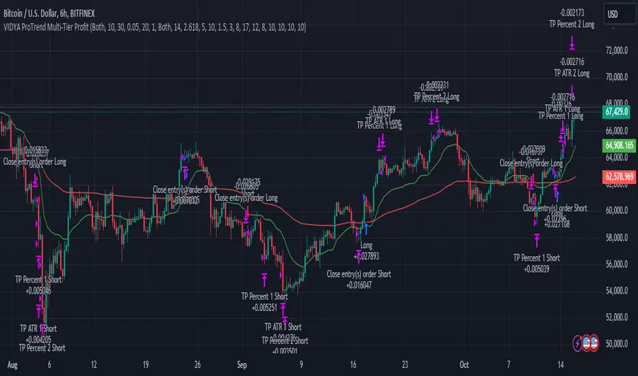
VIDYA ProTrend Multi-Tier ProfitHello! This time is about a trend-following system.
VIDYA is quite an interesting indicator that adjusts dynamically to market volatility, making it more responsive to price changes compared to traditional moving averages. Balancing adaptability and precision, especially with the more aggressive short trade settings, challenged me to fine-tune the strategy for a variety of market conditions.
█ Introduction and How it is Different
The "VIDYA ProTrend Multi-Tier Profit" strategy is a trend-following system that combines the VIDYA (Variable Index Dynamic Average) indicator with Bollinger Bands and a multi-step take-profit mechanism.
Unlike traditional trend strategies, this system allows for more adaptive profit-taking, adjusting for long and short positions through distinct ATR-based and percentage-based targets. The innovation lies in its dynamic multi-tier approach to profit-taking, especially for short trades, where more aggressive percentages are applied using a multiplier. This flexibility helps adapt to various market conditions by optimizing trade management and profit allocation based on market volatility and trend strength.
BTCUSD 6hr performance
█ Strategy, How it Works: Detailed Explanation
The core of the "VIDYA ProTrend Multi-Tier Profit" strategy lies in the dual VIDYA indicators (fast and slow) that analyze price trends while accounting for market volatility. These indicators work alongside Bollinger Bands to filter trade entries and exits.
🔶 VIDYA Calculation
The VIDYA indicator is calculated using the following formula:
Smoothing factor (𝛼):
alpha = 2 / (Length + 1)
VIDYA formula:
VIDYA(t) = alpha * k * Price(t) + (1 - alpha * k) * VIDYA(t-1)
Where:
k = |Chande Momentum Oscillator (MO)| / 100
🔶 Bollinger Bands as a Volatility Filter
Bollinger Bands are calculated using a rolling mean and standard deviation of price over a specified period:
Upper Band:
BB_upper = MA + (K * stddev)
Lower Band:
BB_lower = MA - (K * stddev)
Where:
MA is the moving average,
K is the multiplier (typically 2), and
stddev is the standard deviation of price over the Bollinger Bands length.
These bands serve as volatility filters to identify potential overbought or oversold conditions, aiding in the entry and exit logic.
🔶 Slope Calculation for VIDYA
The slopes of both fast and slow VIDYAs are computed to assess the momentum and direction of the trend. The slope for a given VIDYA over its length is:
Slope = (VIDYA(t) - VIDYA(t-n)) / n
Where:
n is the length of the lookback period. Positive slope indicates bullish momentum, while negative slope signals bearish momentum.
LOCAL picture
🔶 Entry and Exit Conditions
- Long Entry: Occurs when the price moves above the slow VIDYA and the fast VIDYA is trending upward. Bollinger Bands confirm the signal when the price crosses the upper band, indicating bullish strength.
- Short Entry: Happens when the price drops below the slow VIDYA and the fast VIDYA trends downward. The signal is confirmed when the price crosses the lower Bollinger Band, showing bearish momentum.
- Exit: Based on VIDYA slopes flattening or reversing, or when the price hits specific ATR or percentage-based profit targets.
🔶 Multi-Step Take Profit Mechanism
The strategy incorporates three levels of take profit for both long and short trades:
- ATR-based Take Profit: Each step applies a multiple of the ATR (Average True Range) to the entry price to define the exit point.
The first level of take profit (long):
TP_ATR1_long = Entry Price + (2.618 * ATR)
etc.
█ Trade Direction
The strategy offers flexibility in defining the trading direction:
- Long: Only long trades are considered based on the criteria for upward trends.
- Short: Only short trades are initiated in bearish trends.
- Both: The strategy can take both long and short trades depending on the market conditions.
█ Usage
To use the strategy effectively:
- Adjust the VIDYA lengths (fast and slow) based on your preference for trend sensitivity.
- Use Bollinger Bands as a filter for identifying potential breakout or reversal scenarios.
- Enable the multi-step take profit feature to manage positions dynamically, allowing for partial exits as the price reaches specified ATR or percentage levels.
- Leverage the short trade multiplier for more aggressive take profit levels in bearish markets.
This strategy can be applied to different asset classes, including equities, forex, and cryptocurrencies. Adjust the input parameters to suit the volatility and characteristics of the asset being traded.
█ Default Settings
The default settings for this strategy have been designed for moderate to trending markets:
- Fast VIDYA Length (10): A shorter length for quick responsiveness to price changes. Increasing this length will reduce noise but may delay signals.
- Slow VIDYA Length (30): The slow VIDYA is set longer to capture broader market trends. Shortening this value will make the system more reactive to smaller price swings.
- Minimum Slope Threshold (0.05): This threshold helps filter out weak trends. Lowering the threshold will result in more trades, while raising it will restrict trades to stronger trends.
Multi-Step Take Profit Settings
- ATR Multipliers (2.618, 5.0, 10.0): These values define how far the price should move before taking profit. Larger multipliers widen the profit-taking levels, aiming for larger trend moves. In higher volatility markets, these values might be adjusted downwards.
- Percentage Levels (3%, 8%, 17%): These percentage levels define how much the price must move before taking profit. Increasing the percentages will capture larger moves, while smaller percentages offer quicker exits.
- Short TP Multiplier (1.5): This multiplier applies more aggressive take profit levels for short trades. Adjust this value based on the aggressiveness of your short trade management.
Each of these settings directly impacts the performance and risk profile of the strategy. Shorter VIDYA lengths and lower slope thresholds will generate more trades but may result in more whipsaws. Higher ATR multipliers or percentage levels can delay profit-taking, aiming for larger trends but risking partial gains if the trend reverses too early.
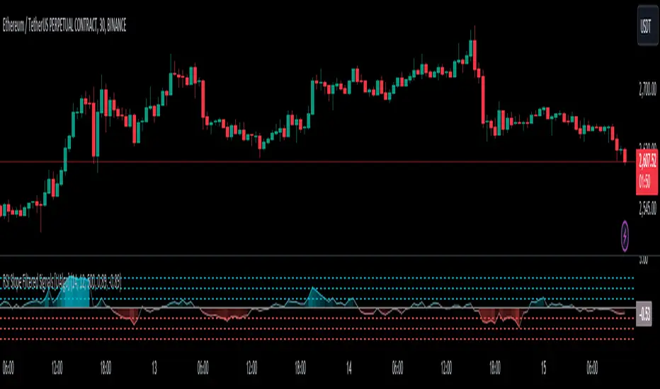
RSI Slope Filtered Signals [UAlgo]The "RSI Slope Filtered Signals " is a technical analysis tool designed to enhance the accuracy of RSI (Relative Strength Index) signals by incorporating slope analysis. This indicator not only considers the RSI value but also analyzes the slope of the RSI over a specified number of bars, providing a more refined signal that accounts for the momentum and trend strength. By utilizing both positive and negative slope arrays, the indicator dynamically adjusts its thresholds, ensuring that signals are responsive to changing market conditions. This tool is particularly useful for traders looking to identify overbought and oversold conditions with a higher degree of precision, filtering out noise and providing clear visual cues for potential market reversals.
🔶 Key Features
Dynamic Slope Analysis: Measures the slope of RSI over a customizable number of bars, offering insights into the momentum and trend direction.
Adaptive Thresholds: Uses historical slope data to calculate dynamic thresholds, adjusting signal sensitivity based on market conditions.
Normalized Slope Calculation: Normalizes the slope values to provide a consistent measure across different market conditions, making the indicator more versatile.
Clear Signal Visualization: The indicator plots both positive and negative normalized slopes with color gradients, visually representing the strength of the trend.
Overbought and Oversold Signals: Plots overbought and oversold signals directly on the chart when the calculated value reaches the user-specified threshold, helping traders identify potential reversal points.
Customizable Settings: Allows users to adjust the RSI length, slope measurement bars, and lookback periods, providing flexibility to tailor the indicator to different trading strategies.
🔶 Interpreting the Indicator
The "RSI Slope Filtered Signals " indicator is designed to be easy to interpret. Here's how you can use it:
Normalized Slope: The indicator plots the normalized slope of the RSI, with values above zero indicating positive momentum and values below zero indicating negative momentum. A higher positive slope suggests a strong upward trend, while a deeper negative slope indicates a strong downward trend.
Reversal Signals: The indicator plots several horizontal lines at different thresholds (+3, +2, +1, 0, -1, -2, -3). These levels are used to gauge the strength of the momentum based on the normalized slope. For example, a normalized slope crossing above the +2 threshold may indicate a strong bullish trend, while crossing below the -2 threshold may suggest a strong bearish trend. These thresholds help in understanding the intensity of the current trend and provide context for interpreting the indicator's signals.
This indicator generates overbought and oversold signals not solely based on the RSI entering extreme levels (above 70 for overbought and below 30 for oversold), but also by considering the behavior of the normalized slope relative to specific thresholds. Specifically, the Overbought Signal (🔽) is triggered when the RSI is above 70 and the normalized slope from the previous bar is greater than or equal to the upper threshold, with the current slope being lower than the previous slope, indicating a potential bearish reversal as momentum may be slowing down.
Similarly, the Oversold Signal (🔼) is generated when the RSI is below 30 and the normalized slope from the previous bar is less than or equal to the lower threshold, with the current slope being higher than the previous slope, signaling a potential bullish reversal as the downward momentum may be weakening.
Area Plots: The indicator also plots the positive and negative slopes as filled areas, providing a quick visual cue for the strength and direction of the trend. Green areas represent positive slopes (upward momentum), while red areas represent negative slopes (downward momentum).
By combining these elements, the "RSI Slope Filtered Signals " provides a comprehensive view of the market's momentum, helping traders make more informed decisions by filtering out false signals and focusing on the significant trends.
🔶 Disclaimer
Use with Caution: This indicator is provided for educational and informational purposes only and should not be considered as financial advice. Users should exercise caution and perform their own analysis before making trading decisions based on the indicator's signals.
Not Financial Advice: The information provided by this indicator does not constitute financial advice, and the creator (UAlgo) shall not be held responsible for any trading losses incurred as a result of using this indicator.
Backtesting Recommended: Traders are encouraged to backtest the indicator thoroughly on historical data before using it in live trading to assess its performance and suitability for their trading strategies.
Risk Management: Trading involves inherent risks, and users should implement proper risk management strategies, including but not limited to stop-loss orders and position sizing, to mitigate potential losses.
No Guarantees: The accuracy and reliability of the indicator's signals cannot be guaranteed, as they are based on historical price data and past performance may not be indicative of future results.
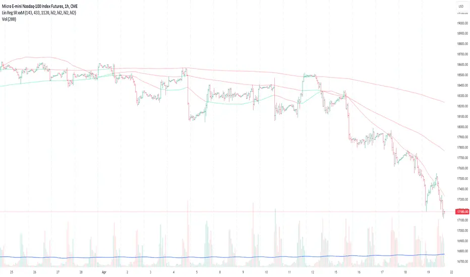
Lin Reg (Linear Regression) Support and Resistance by xxMargauxLin Reg (Linear Regression) Support & Resistance by xxMargaux 💸
This indicator plots three linear regression lines (Lin Reg) on the price chart, providing insights into potential support and resistance levels. It calculates Lin Reg lines based on user-defined lengths and sources.
This indicator's settings were initially configured for MNQ1! (E-Mini Nasdaq 100 futures contracts). But works as intended on any security and on any timeframe.
When price is below a given Lin Reg line, that line will be red and may serve as resistance as price moves up towards the line. That is, it may be a potential short entry opportunity. When price is above a given Lin Reg line, that line will be green and may serve as support as price continues up from the line. That is, it may be a potential long entry opportunity.
When price starts to break sideways or down through the Lin Reg lines, this may signal a reversal from uptrend to downtrend. When price starts to break sideways or up through the Lin Reg Lines, this may signal a reversal from downtrend to uptrend. In very strong trends, breaking through the lines briefly may provide an entry opportunity, but be cautious because a trend reversal may also be possible.
Inputs:
Length of Price Lin Reg Lines: Customize the lengths of the three Lin Reg lines.
Source for Price Lin Reg Lines: Choose the source for each Lin Reg line.
Source for Security Price: Select the price source for the security.
Features:
Trend Analysis: Assists in visualizing price trends based on the relationship between the security price and Lin Reg lines, which will be colored according to whether price is above or below each Lin Reg line.
Customizable Colors: When price is above a Lin Reg line that line will be green. When price is below a Lin Reg line, that line will be red.
Here's a beginner-friendly explanation of linear regression lines 💡
Best-Fit Line: Imagine you have a scatter plot of closing prices on a chart. Linear regression aims to find the straight line that best fits the overall trend of these data points. It's like drawing a line through the center of the data that minimizes the distance between the line and each data point.
Trend Identification: Once the linear regression line is plotted on a price chart, it provides a visual representation of the trend. If the price is generally rising, the linear regression line will slope upwards. If the price is falling, the line will slope downwards. This helps traders identify whether the trend is bullish (upward) or bearish (downward).
Support and Resistance: Linear regression lines can also act as dynamic support and resistance levels. When the price is above the linear regression line, it may act as support, meaning the price tends to bounce off the line and continue higher. Conversely, when the price is below the line, it may act as resistance, with the price encountering selling pressure and potentially reversing lower.
Reversal Signals: Changes in the slope or direction of the linear regression line can signal potential trend reversals. For example, if the price breaks above a downward-sloping linear regression line, it may indicate a shift from a downtrend to an uptrend, and vice versa.
Adjustable Parameters: Traders can customize the length of the linear regression line by adjusting the period over which it's calculated. Shorter periods may be more sensitive to recent price changes, while longer periods may provide a smoother trend line.
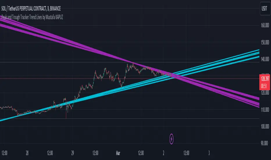
Peak and Trough Tracker by Mustafa KAPUZPeak and Trough Tracker
This indicator identifies the highest and lowest prices reached in two user-defined time periods. It then draws two lines connecting these peak and trough points. The purple line represents the connection between the highest prices, while the aqua line represents the relationship between the lowest prices. Both lines extend into the future and past, providing insights into potential support and resistance levels.
How to Use:
Add the indicator to your chart.
Enter two time periods.
Analyze the lines connecting peak and trough points.
This tool helps visually understand the market's key turning points and adjust your investment strategy based on these insights.
Zirve ve Dip Noktaları İzleyici
Bu indikatör, kullanıcı tarafından belirlenen iki zaman periyodunda piyasanın ulaştığı en yüksek ve en düşük fiyatları tespit eder. Ardından, bu zirve ve dip noktalarını birleştiren iki çizgi çizer. Mor çizgi, en yüksek fiyatlar arasındaki bağlantıyı gösterirken; aqua çizgi, en düşük fiyatlar arasındaki ilişkiyi temsil eder. Her iki çizgi de geleceğe ve geçmişe doğru uzanarak, potansiyel destek ve direnç seviyeleri hakkında fikir verir.
Kullanımı:
İndikatörü grafik üzerine ekleyin.
İki zaman periyodu girin.
Zirve ve dip noktalarını birleştiren çizgilerin analizini yapın.
Bu araç, piyasanın önemli dönüm noktalarını görsel olarak anlamanıza ve yatırım stratejinizi bu bilgilere göre ayarlamanıza yardımcı olur.
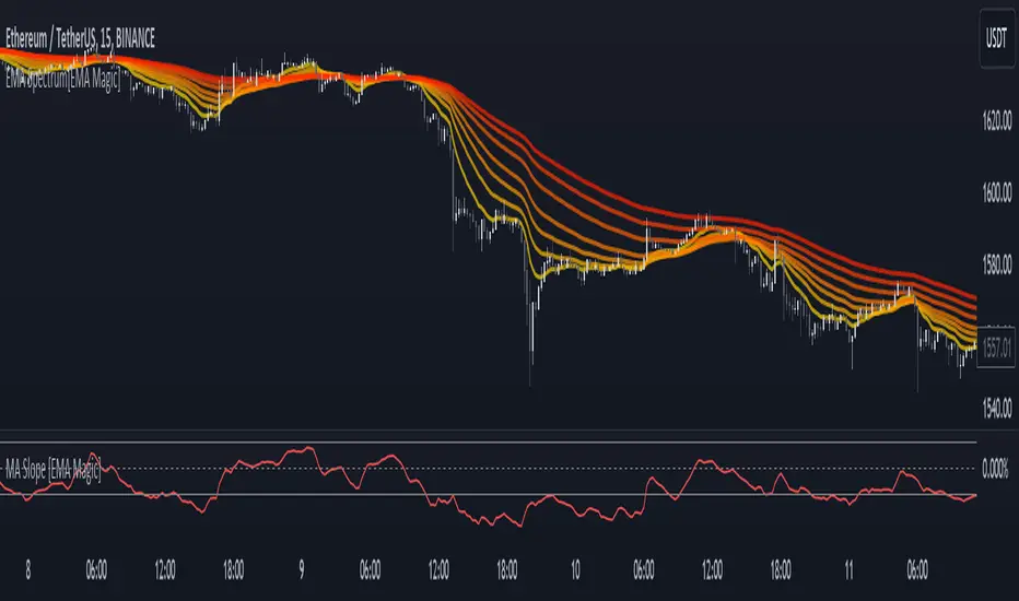
MA Slope [EMA Magic]█ Overview:
The MA Slope calculates the slope based on a given moving average.
The Moving Average Slope indicator allows you to identify the direction and the strength of a trend.
It calculates the rate of change in percentage based on the user-defined moving average.
█ Calculation: This indicator calculates the slope based on the changes of moving average and normalizes it with Average True Range(ATR).
The default value of ATR is 7.I recommend not changing it unless you know exactly what are you doing.
█ Input Settings:
The settings are divided into three sections:
The first section is for time frame adjustments. Modify it separately from the chart, Allows you to use moving averages from different time frames.
In the second section, you can configure the base calculation,including Moving Average and Average True Range(ATR) settings.
In the third section, you can detect breakout and sudden change signals, which are highlighted in the background of the indicator.
Note that When you change the breakout limit value, it also affects the band limit indicator on your chart.
To avoid signal confusion, use only one at a time.
Here is the example the breakout signals:
█ Usage:
When the slope is increasing, it indicates an uptrend.
When the slope is decreasing, it indicates a downtrend.
When the slope is moving around zero and choppy, it indicates no specific trend or price is in a range zone.
Uptrend and Range Zone example:
Downtrend example:
Slope peaks on extreme levels can signal a potential trend reversal point.
Breakout of the upper or lower bands can be translated into a trading signal.Indicating that price will probably continue to move in the direction of the breakout.
Favor long setups when the slope is increasing or it is positive and favor short setups when the slope is decreasing or it is negative.
Fits with any moving average you use, e.g., EMA, WMA, MA Ribbon, and more.
█ Alert
Alerts are available for both signal conditions.
█ Recap
Take the time to study price movements alongside this indicator for a deeper understanding.Whether you're a novice or experienced trader, this indicator can come helpful
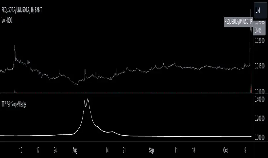
TTP Pair Slope/HedgePair slope/hedge uses linear regression to calculate the hedge ratio (slope) between the two assets within a period.
It allows you to specify a "from" and a "to" candle.
Example:
"A regression from 1000 candles back in time and ignore the last 100 candles. This would result in making a regression of 900 candles in total."
The formula used to perform the regression with the assts X and Y is:
Hedge =
mean( (X-mean(X))^2 )
——————————————————
mean( (X-mean(X)) * (Y-mean(Y)) )
You can later use the hedge in a chart of X - Hedge * Y
(Confirm with 1 / hedge )
If the plot is stationary the period tested should look like stationary.
If you cross an imaginary horizontal line across all the values in the period used it should look like a flat channel with values crossing above and below the line.
The purpose of this indicator is to help finding the linear regression test used for conintegration analysis. Conintegration assets is one of the requirements to consider assets for pair and hedge trading.
TTP VIX SpyTTP VIX Spy is an indicator that uses data from TVC:VIX to better time entries in the market.
The assumption used is that when the VIX is coming down from the top of its range then the risk on assets can move to the upside and when the VIX is is pushing higher there's a high likelihood or risk on assets going down.
This indicator observes the momentum of VIX using MACD. It offers two different signals both for longs and shorts: signal 1 and 2.
Signal 1 is activate when the begging of a new trend for the VIX is confirmed.
Signal 2 is activated when the VIX pulls back from an extreme value.
You can configure the parameters of the internal super trend and the look back for the slope applied to price and RSIs.
The indicator offers the following filter parameters:
- Price RSI slope: it filters signals that have RSI slope pointing in the opposite direction of the signal.
- Counter trend: it filters signals that are not counter trending super trend.
- Wide BBW: it filters signals that happen when there hasn't been high price volatility
- Price slope: it filters signals when the price is not pointing in the direction of the signal (buy: up, sell: down)
- VIX RSI filter: it filters VIX RSI values overextended. MACD can be in the right range, but sometimes RSI contradicts it. By default is OFF since it can cause false negatives.
- Working days only: it filters signals that occur in the weekend.
The colours below the price action show how the VIX momentum is changing. Transitions from red into pink and then green show how the fear is fading which tends to lead to lead to bullish moves, and the opposite when the transitions are from green to red.
Performance and initial thoughts.
I have tried VIX Spy on both BINANCE:BTCUSDT.P and BINANCE:ETHUSDT.P and it seems to offer a decent win ratio. As you can see I had to add many filter to remove bad entries and left toggles available to decide which ones you want to use.
I tried the signal in the 4H, 1H and 15min with mixed results. I tend to incline for the results in the 1H.
VIX signal offers a backtestable stream and alerts both for signals 1 and 2.

Acceleration-Based MA Slope PredictionHello traders,
I developed this indicator while working on a trading strategy using moving average slope and acceleration, and I found the concept interesting enough to share it.
Let me briefly explain this indicator.
----About White Plot----
1. Calculate the first derivative approximation at the current point of the Moving Average, and then calculate the second derivative approximation to obtain the 'Acceleration'.
2. Where the acceleration is 0, it signifies a change in the force of the moving average.
3. Therefore, by drawing a parabola based on the acceleration at that time, can depict the parabolic shape of the moving average.
This is represented as a white circle on the indicator.
4. These circles are reset at the next point where the acceleration is 0, indicating a change in the parabolic force.
If the moving average rises more sharply than the predicted value of the rising parabola, a more drastic increase is expected.
5. In this case, you can start risk management around the time the drawn parabola breaks.
(The actual MA is represented by green/red lines)
6. Before the trend changes, i.e., before the direction of the moving average changes, there is a section where the acceleration is 0, and this is represented on the chart as follows.
(The lower indicator shows the acceleration of the corresponding parabola)
----About Red Plot----
1. Calculate the first derivative approximation of the moving average value, the 'slope'.
2. Where the slope is 0, it represents the extreme point of the parabola.
3. Therefore, by using the acceleration at that point as the coefficient of the quadratic function and setting the extreme point as a vertex, we can draw a quadratic function. This is represented as a red circle on the indicator.
(Keep in mind that the actual moving average is not a quadratic function; this is a "forced" quadratic function assuming the parabola is maintained)
4. These circles are reset at the next extreme point where the slope is 0, and a new quadratic function is created.
Based on the formula obtained in the above process, you can predict the future moving average through 'offset'.
5. That is, if the x value at the current point is 'k', you can predict the moving average one candle ahead by substituting (k+1) into the quadratic function.
The predicted value at the past position is shown as a red circle.
6. The smoother the chosen moving average, the fewer extreme points will appear, and the higher the likelihood of the parabola fitting.
For the T3 set as the default value, it shows very high accuracy even when predicting about 20 candles ahead.
On the other hand, rough moving averages like SMA have limited prediction value.
(SMA 60, offset = 10)
--------
The moving average with a very high level of accuracy is JMA (Jurik Moving Average). However, since the code for this moving average is not public, I recommend those interested to check it through my code.
Additionally, I believe the code of this indicator I've uploaded has significant utility.
As an example, you can use the breaking point of the parabola predicted by the acceleration to determine when the force changes again for entries/losses. There are many other possible applications as well.
I look forward to seeing more excellent results from this indicator.
--------
안녕하세요 트레이더여러분.
이 지표는, 제가 이동평균선의 기울기와 가속도를 이용하여 매매를 하기 위한 지표를 개발하다가, 흥미로운 내용이라고 판단하여 만들게 되었습니다.
이 지표에 대해 간단히 설명드리겠습니다.
----하얀색 플롯에 대해----
1. 이동평균선이 진행되는 현재 시점에서 미분의 근사값을 구하고, 다시 한 번 미분의 근사값을 구해서 '가속도'를 얻습니다.
2. 가속도가 0이 되는 곳은, 곧 해당 이동평균선의 힘이 바뀌는 곳을 의미합니다.
3. 따라서, 그 당시 시점 기준으로 포물선을 그려낸다면, 가속도를 이용하여 해당 이동평균선의 포물선을 그려낼 수 있습니다. 이것은 지표의 하얀색점로서 표기됩니다.
4. 이 때, 이러한 점들은 다음의 가속도가 0이 되는 지점, 즉 포물선의 힘이 바뀌는 곳에서 다시 초기화됩니다.
5. 올라가고 있던 포물선에서의 예측치보다 이동평균선이 더 급하게 올라간다면, 더욱 급격한 상승이 예상됩니다. 이 경우, 그려지고있는 포물선이 깨질 때쯤부터 리스크 관리를 시작할 수 있습니다.
(녹색/빨간색의 선으로 실제 MA를 표현했습니다. 거슬리시면 '모습'가셔서 끄셔도 좋습니다. )
6. 추세가 변경되기 전, 즉 이동평균선의 방향이 바뀌기 전에는 가속도가 0이 되는 구간이 존재하고, 그것이 차트 위에 다음과같이 표현됩니다.
(하단의 지표는, 해당 포물선의 가속도을 나타냅니다)
----붉은색 플롯에 대해----
1. 이동평균선 값을 미분 근사값 즉, '기울기'를 구합니다.
2. 기울기가 0이 되는 곳은, 포물선이 극점이 되는 곳을 뜻합니다.
3. 따라서, 해당 시점의 가속도를 2차함수의 계수로 하여, 또한 해당 극점을 하나의 꼭지점으로 설정하여,이차함수를 그려낼 수 있습니다. 이것은 지표의 빨간색점으로서 표현됩니다.
(실제 이동평균선은 2차함수가 아니기에, 포물선이 유지된다는 가정 하에 "억지로"만들어낸 이차함수입니다)
4. 이 때, 이러한 점은 다음 극점이 0이 되는 곳에서 초기화되고 이차함수가 만들어집니다.
5. 위의 과정에서 얻은 식을 바탕으로 'offset'을 통해 미래의 이동평균선을 예측할 수 있습니다.
즉, 현재시점의 x값을 'k'라고 한다면, (k+1)을 이차함수에 대입하여 1캔들 앞의 이동평균선을 예측할 수 있습니다.
해당 예측치가 지나간 자리는, 빨간색점을 통해 보여집니다.
6. 선택한 이동평균선이 스무스할수록 극점은 덜 등장하게되고, 포물선의 위치가 맞아들어갈 가능성이 높습니다.
현재 디폴트값으로 설정된 T3의 경우, 약 20캔들 앞을 예측해도 매우 높은 정확도를 보여줍니다.
반면에, SMA와 같이 울퉁불퉁한 이동평균선은 가능한 예측치가 크지 않습니다.
(SMA 60, offset=10)
--------
매우 높은 수준의 정확도를 보여준 이동평균선은 JMA(Jurik Moving Average)입니다. 다만 이 이동평균선은 코드가 공개되지 않았기때문에, 관심있으신 분은 저의 코드를 통해 한번 확인해보시길 권장드립니다.
추가로, 제가 올린 이 지표의 코드는 이용가치가 높다고 생각합니다.
하나의 예시로서, 가속도로 예측한 포물선이 깨지는 곳을 기준으로, 힘이 다시 한 번 바뀌는 것을 이용해 진입/로스를 할 수 있습니다. 그 외에도 매우 다양한 활용이 가능합니다.
이 지표를 통해 더욱 좋은 새로운 결과물이 나오길 기대해봅니다.

Rainbow Collection - BlueSlopes are an increasingly key concept in Technical Analysis. The most basic type is to calculate them on the prices, but also on technical indicators such as moving averages and the RSI.
In technical analysis, you generally use the RSI to detect imminent reversal moves within a range. In the case of the Blue indicator, we are calculating the slope of the market price and then calculating the RSI of that slope in order to detect instances of reversal.
The Blue indicator is therefore used as follows:
* A bullish signal is generated whenever the 21-period RSI of the 21-period market slope surpasses 30 after having been below it but remains below 35.
*A bearish signal is generated whenever the 21-period RSI of the 21-period market slope breaks 70 after having been above it but remains above 65.
The aim of the Blue indicator is to capture reversals as early as possible through a combination of slopes and entry techniques.

Leavitt Convolution Acceleration [CC]The Leavitt Convolution Slope indicator was created by Jay Leavitt (Stocks and Commodities Oct 2019, page 11), who is most well-known for creating the Volume-Weighted Average Price indicator. This indicator didn't have a good explanation or description so I custom-coded most of it. The way it works is it will give trend spikes in the direction of the underlying trend. If you don't see a spike then it means that the stock isn't trending at the moment. One possible avenue to explore with this indicator is judging the size of the trend spike before you open a position in that direction (or the opposite direction if you are shorting). I added a normalization function using code from a good friend @loxx that I recommend leaving on but feel free to experiment with it. I have color coded the lines to turn light green for a standard buy signal or dark green for a strong buy signal and light red for a standard sell signal, and dark red for a strong sell signal.
This is another indicator in a series that I'm publishing to fulfill a special request from @ashok1961 so let me know if you ever have any special requests for me.
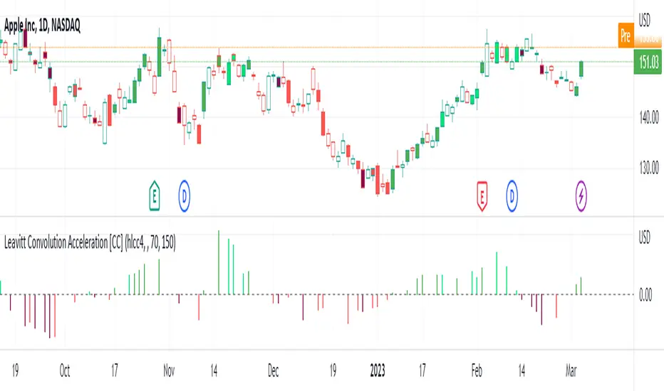
Slope NormalizerBrief:
This oscillator style indicator takes another indicator as its source and measures the change over time (the slope). It then isolates the positive slope values from the negative slope values to determine a 'normal' slope value for each.
** A 'normal' value of 1.0 is determined by the average slope plus the standard deviation of that slope.
The Scale
This indicator is not perfectly linear. The values are interpolated differently from 0.0 - 1.0 than values greater than 1.0.
From values 0.0 to 1.0 (positive or negative): it means that the value of the slope is less than 'normal' **.
Any value above 1.0 means the current slope is greater than 'normal' **.
A value of 2.0 means the value is the average plus 2x the standard deviation.
A value of 3.0 means the value is the average plus 3x the standard deviation.
A value greater than 4.0 means the value is greater than the average plus 4x the standard deviation.
Because the slope value is normalized, the meaning of these values can remain generally the same for different symbols.
Potential Usage Examples/b]
Using this in conjunction with an SMA or WMA may indicate a change in trend, or a change in trend-strength.
Any values greater than 4 indicate a very strong (and unusual) trend that may not likely be sustainable.
Any values cycling between +1.0 and -1.0 may mean indecision.
A value that is decreasing below 0.5 may predict a change in trend (slope may soon invert).
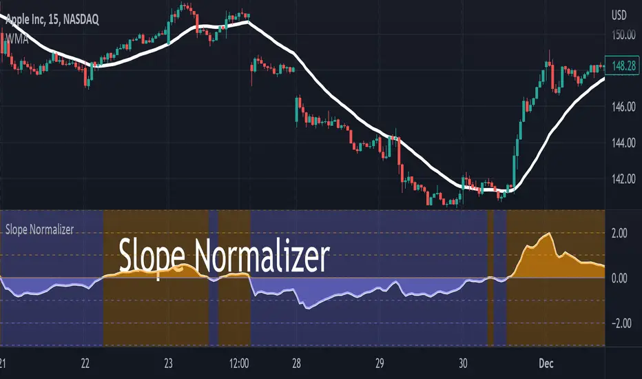
Slope_TKLibrary "Slope_TK"
This library calculate the slope of a serie between two points
The serie can be ta.ema(close,200) for example
The size is the number of bars between the two points for the slope calculation, for example it can be 10
slope_of_ema200 = slope(t a.eam(close, 200) , 10 )
slope( float serie, int size )
Trend Slope Meter - KaspricciTrend Slope Meter
This indicator measures the slope of the trend defined by a moving average or an external source. The slope is calculated by the change of price in ticks for a defined number of bars divided by the number of bars.
Settings
Source - Default: close price. Used to calculate the moving average as basis for slope measurement. Can be an external source of a different indicator as well. In case you select an external source, you can disable the moving average calculation.
Moving Average Settings
Type - Default: EMA. Type of moving average calculation. All provided out of the box by TradingView.
Length - Default: 50. Length used to calculate moving average.
Slope Settings
Length - Default: 50. Length used to calculate slope.

Directional Slope Strength IndexThe most basic of trend indicators is the price change over some period of time. Rate of change is the most common indicator to use which calculates the current price minus the price n bars back. I've written this indicator to solve several problems the default value of ROC.
1. We're interested in the magnitude or strength of the slope of change.
2. We need a number that we can make decisions from between 0 and something close to a peak of 10.
3. We need the ability to define a threshold where a directional change might be taking place.
The Directional Slope Strength Index solves these problems by taking 1000 samples of your given Rate of Change input and calculating a standard score (or z-score) which represents the number of standard deviations by which the current rate of change is above or below the historical average. A higher number represents a stronger move up and a lower (negative) number represents a stronger move down. A value closer to 0 would represent a sideways trend or the slowing of a current trend.
A potential threshold could be 2 or -2 which is two standard deviations from the mean ROC.
The inputs can be modified to control the sensitivity.
1. A lower ROC length would provide a more sensitive measure, but still measure how that sensitive input changes over 1000 samples.
2. I recommend keeping the sample rate at 1000 as that provides enough historical data to give a more accurate distribution and therefore a more accurate DSSI (z-score).
A number of decisions can be made from the indicator:
1. When the DSSI crosses above 2, it could be a sign of a strong move upward. When below -2 it could be a sign of a strong downward move.
2. When the DSSI persists in a positive or negative channel between 0 and 2 or 0 and -2 this could indicate the formation of the next trend.
3. Values outside 2 and -2 standard deviations should be interpreted as high volatility environments.
4. For convenience, a highest and lowest DSSI have been plotted to provide references to the historical extremes.
I'm open to any questions and feedback as this is a first, original indicator for me.

Clutter Fitler [Loxx]Clutter Fitler is a simple indicator to demonstrate a clutter filter. The purpose of this technique is to filter useless noise.
What is a Clutter Filter?
For our purposes here, this is a filter that compares the slope of the trading filter output to a threshold to determine whether to shift trends. If the slope is up but the slope doesn't exceed the threshold, then the color is gray and this indicates a chop zone. If the slope is down but the slope doesn't exceed the threshold, then the color is gray and this indicates a chop zone. Alternatively if either up or down slope exceeds the threshold then the trend turns green for up and red for down. Fro demonstration purposes, an EMA is used as the moving average. This filtering technique will be used for future indicators.
Included
Bar coloring
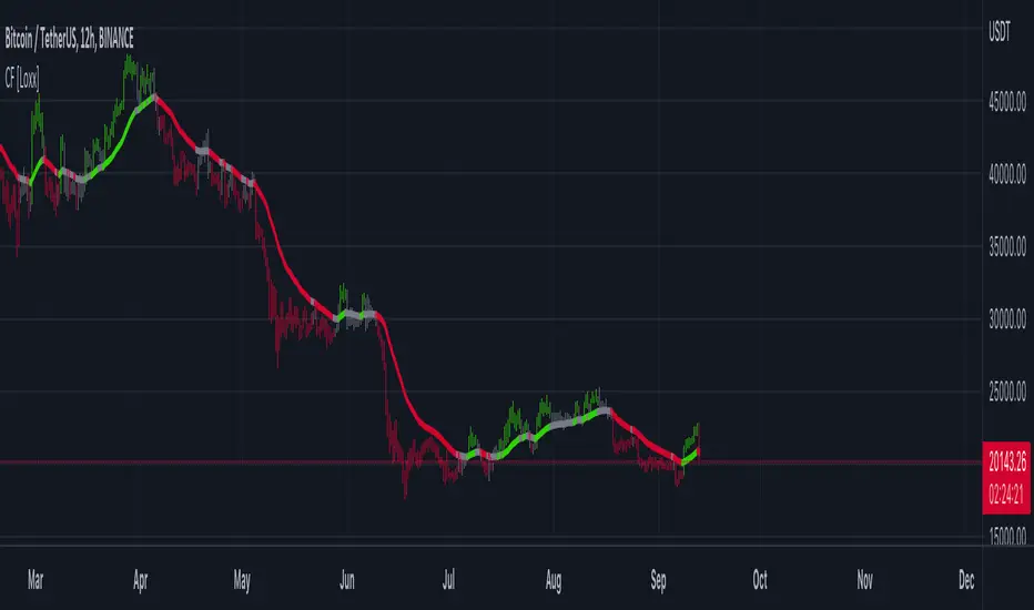
Multi TF Trend Indicator
...Mark Douglas in his book Trading in the Zone wrote
The longer the time frame, the more significant the trend, so a trending market on a daily bar chart is more significant than a trending market on a 30-minute bar chart. Therefore, the trend on the daily bar chart would take precedence over the trend on the 30-minute bar chart and would be considered the major trend. To determine the direction of the major trend, look at what is happening on a daily bar chart. If the trend is up on the daily, you are only going to look for a sell-off or retracement down to what your edge defines as support on the 30-minute chart. That's where you will become a buyer. On the other hand, if the trend is down on the daily, you are only going to look for a rally up to what your edge defines as a resistance level to be a seller on the 30-minute chart. Your objective is to determine, in a downtrending market, how far it can rally on an intraday basis and still not violate the symmetry of the longer trend. In an up-trending market, your objective is to determine how far it can sell off on an intraday basis without violating the symmetry of the longer trend. There's usually very little risk associated with these intraday support and resistance points, because you don't have to let the market go very far beyond them to tell you the trade isn't working.
The purpose of this indicator to show both the major and minor trend on the same chart with no need to switch between timeframes
Script includes
timeframe to determine the major trend
price curve, close price is default, but you can pick MA you want
type of coloring, either curve color or the background color
Implementation details
major trend is determined by the slope of the price curve
Further improvements
a variation of techniques for determining the major trend (crossing MA, pivot points etc.)
major trend change alerts
Thanks @loxx for pullData helper function
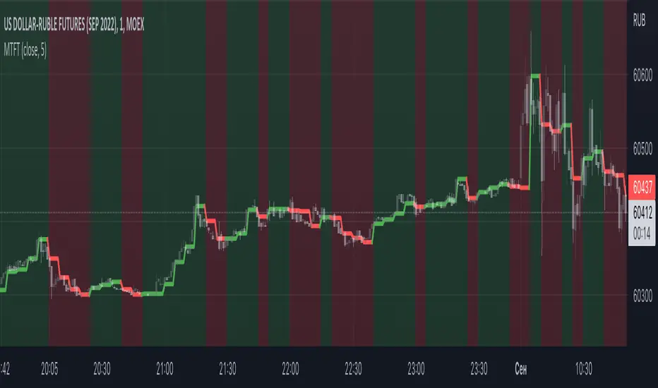
HMA Slope Variation [Loxx]HMA Slope Variation is an indicator that uses HMA moving average to calculate a slope that is then weighted to derive a signal.
The center line
The center line changes color depending on the value of the:
Slope
Signal line
Threshold
If the value is above a signal line (it is not visible on the chart) and the threshold is greater than the required, then the main trend becomes up. And reversed for the trend down.
Colors and style of the histogram
The colors and style of the histogram will be drawn if the value is at the right side, if the above described trend "agrees" with the value (above is green or below zero is red) and if the High is higher than the previous High or Low is lower than the previous low, then the according type of histogram is drawn.
What is the Hull Moving Average?
The Hull Moving Average ( HMA ) attempts to minimize the lag of a traditional moving average while retaining the smoothness of the moving average line. Developed by Alan Hull in 2005, this indicator makes use of weighted moving averages to prioritize more recent values and greatly reduce lag.
Included
Alets
Signals
Bar coloring
Loxx's Expanded Source Types

T3 Slope Variation [Loxx]T3 Slope Variation is an indicator that uses T3 moving average to calculate a slope that is then weighted to derive a signal.
The center line
The center line changes color depending on the value of the:
Slope
Signal line
Threshold
If the value is above a signal line (it is not visible on the chart) and the threshold is greater than the required, then the main trend becomes up. And reversed for the trend down.
Colors and style of the histogram
The colors and style of the histogram will be drawn if the value is at the right side, if the above described trend "agrees" with the value (above is green or below zero is red) and if the High is higher than the previous High or Low is lower than the previous low, then the according type of histogram is drawn.
What is the T3 moving average?
Better Moving Averages Tim Tillson
November 1, 1998
Tim Tillson is a software project manager at Hewlett-Packard, with degrees in Mathematics and Computer Science. He has privately traded options and equities for 15 years.
Introduction
"Digital filtering includes the process of smoothing, predicting, differentiating, integrating, separation of signals, and removal of noise from a signal. Thus many people who do such things are actually using digital filters without realizing that they are; being unacquainted with the theory, they neither understand what they have done nor the possibilities of what they might have done."
This quote from R. W. Hamming applies to the vast majority of indicators in technical analysis . Moving averages, be they simple, weighted, or exponential, are lowpass filters; low frequency components in the signal pass through with little attenuation, while high frequencies are severely reduced.
"Oscillator" type indicators (such as MACD , Momentum, Relative Strength Index ) are another type of digital filter called a differentiator.
Tushar Chande has observed that many popular oscillators are highly correlated, which is sensible because they are trying to measure the rate of change of the underlying time series, i.e., are trying to be the first and second derivatives we all learned about in Calculus.
We use moving averages (lowpass filters) in technical analysis to remove the random noise from a time series, to discern the underlying trend or to determine prices at which we will take action. A perfect moving average would have two attributes:
It would be smooth, not sensitive to random noise in the underlying time series. Another way of saying this is that its derivative would not spuriously alternate between positive and negative values.
It would not lag behind the time series it is computed from. Lag, of course, produces late buy or sell signals that kill profits.
The only way one can compute a perfect moving average is to have knowledge of the future, and if we had that, we would buy one lottery ticket a week rather than trade!
Having said this, we can still improve on the conventional simple, weighted, or exponential moving averages. Here's how:
Two Interesting Moving Averages
We will examine two benchmark moving averages based on Linear Regression analysis.
In both cases, a Linear Regression line of length n is fitted to price data.
I call the first moving average ILRS, which stands for Integral of Linear Regression Slope. One simply integrates the slope of a linear regression line as it is successively fitted in a moving window of length n across the data, with the constant of integration being a simple moving average of the first n points. Put another way, the derivative of ILRS is the linear regression slope. Note that ILRS is not the same as a SMA ( simple moving average ) of length n, which is actually the midpoint of the linear regression line as it moves across the data.
We can measure the lag of moving averages with respect to a linear trend by computing how they behave when the input is a line with unit slope. Both SMA (n) and ILRS(n) have lag of n/2, but ILRS is much smoother than SMA .
Our second benchmark moving average is well known, called EPMA or End Point Moving Average. It is the endpoint of the linear regression line of length n as it is fitted across the data. EPMA hugs the data more closely than a simple or exponential moving average of the same length. The price we pay for this is that it is much noisier (less smooth) than ILRS, and it also has the annoying property that it overshoots the data when linear trends are present.
However, EPMA has a lag of 0 with respect to linear input! This makes sense because a linear regression line will fit linear input perfectly, and the endpoint of the LR line will be on the input line.
These two moving averages frame the tradeoffs that we are facing. On one extreme we have ILRS, which is very smooth and has considerable phase lag. EPMA has 0 phase lag, but is too noisy and overshoots. We would like to construct a better moving average which is as smooth as ILRS, but runs closer to where EPMA lies, without the overshoot.
A easy way to attempt this is to split the difference, i.e. use (ILRS(n)+EPMA(n))/2. This will give us a moving average (call it IE /2) which runs in between the two, has phase lag of n/4 but still inherits considerable noise from EPMA. IE /2 is inspirational, however. Can we build something that is comparable, but smoother? Figure 1 shows ILRS, EPMA, and IE /2.
Filter Techniques
Any thoughtful student of filter theory (or resolute experimenter) will have noticed that you can improve the smoothness of a filter by running it through itself multiple times, at the cost of increasing phase lag.
There is a complementary technique (called twicing by J.W. Tukey) which can be used to improve phase lag. If L stands for the operation of running data through a low pass filter, then twicing can be described by:
L' = L(time series) + L(time series - L(time series))
That is, we add a moving average of the difference between the input and the moving average to the moving average. This is algebraically equivalent to:
2L-L(L)
This is the Double Exponential Moving Average or DEMA , popularized by Patrick Mulloy in TASAC (January/February 1994).
In our taxonomy, DEMA has some phase lag (although it exponentially approaches 0) and is somewhat noisy, comparable to IE /2 indicator.
We will use these two techniques to construct our better moving average, after we explore the first one a little more closely.
Fixing Overshoot
An n-day EMA has smoothing constant alpha=2/(n+1) and a lag of (n-1)/2.
Thus EMA (3) has lag 1, and EMA (11) has lag 5. Figure 2 shows that, if I am willing to incur 5 days of lag, I get a smoother moving average if I run EMA (3) through itself 5 times than if I just take EMA (11) once.
This suggests that if EPMA and DEMA have 0 or low lag, why not run fast versions (eg DEMA (3)) through themselves many times to achieve a smooth result? The problem is that multiple runs though these filters increase their tendency to overshoot the data, giving an unusable result. This is because the amplitude response of DEMA and EPMA is greater than 1 at certain frequencies, giving a gain of much greater than 1 at these frequencies when run though themselves multiple times. Figure 3 shows DEMA (7) and EPMA(7) run through themselves 3 times. DEMA^3 has serious overshoot, and EPMA^3 is terrible.
The solution to the overshoot problem is to recall what we are doing with twicing:
DEMA (n) = EMA (n) + EMA (time series - EMA (n))
The second term is adding, in effect, a smooth version of the derivative to the EMA to achieve DEMA . The derivative term determines how hot the moving average's response to linear trends will be. We need to simply turn down the volume to achieve our basic building block:
EMA (n) + EMA (time series - EMA (n))*.7;
This is algebraically the same as:
EMA (n)*1.7-EMA( EMA (n))*.7;
I have chosen .7 as my volume factor, but the general formula (which I call "Generalized Dema") is:
GD (n,v) = EMA (n)*(1+v)-EMA( EMA (n))*v,
Where v ranges between 0 and 1. When v=0, GD is just an EMA , and when v=1, GD is DEMA . In between, GD is a cooler DEMA . By using a value for v less than 1 (I like .7), we cure the multiple DEMA overshoot problem, at the cost of accepting some additional phase delay. Now we can run GD through itself multiple times to define a new, smoother moving average T3 that does not overshoot the data:
T3(n) = GD ( GD ( GD (n)))
In filter theory parlance, T3 is a six-pole non-linear Kalman filter. Kalman filters are ones which use the error (in this case (time series - EMA (n)) to correct themselves. In Technical Analysis , these are called Adaptive Moving Averages; they track the time series more aggressively when it is making large moves.
Included
Alets
Signals
Bar coloring
Loxx's Expanded Source Types