Volatility

Pre-Market & Previous Day Levels 300here is the indicator pre market high low and prev day hihg low levels

Ghost Month HighlighterGhost Month and Trading: Understanding the Phenomenon
Ghost Month (鬼月) is the seventh month of the lunar calendar in Chinese culture, typically falling between late July and September. During this period, it's believed that the gates of the afterlife open and spirits roam the earth. This deeply rooted cultural belief has significant implications for Asian markets, particularly in regions with large Chinese populations like Taiwan, Hong Kong, Singapore, and mainland China.
Why Markets Often Decline or Stay Flat During Ghost Month:
Reduced Business Activity : Many businesses avoid launching new products, signing major contracts, or making significant investments during this period, believing it brings bad luck.
Property Market Slowdown : Real estate transactions drop significantly as people avoid moving homes or making large purchases. In some markets, property sales can decline by 20-30%.
IPO and M&A Drought : Companies often delay IPOs and merger announcements until after Ghost Month, reducing market catalysts.
Retail Spending Drops : Consumer spending on big-ticket items decreases, though spending on offerings and religious items increases.
Self-Fulfilling Prophecy : Many traders and investors reduce positions or stay on the sidelines, creating lower volumes and increased volatility. This becomes a self-fulfilling prophecy where expectation of poor performance leads to actual underperformance.
Tourism and Entertainment Impact : Travel and entertainment sectors see reduced activity as people avoid unnecessary trips and celebrations.
Historical data shows that Asian equity markets often underperform during Ghost Month, with some studies indicating average returns can be 2-5% lower than other months. However, this also creates opportunities for contrarian investors who buy during the seasonal weakness.
Inspired by @honey_xbt

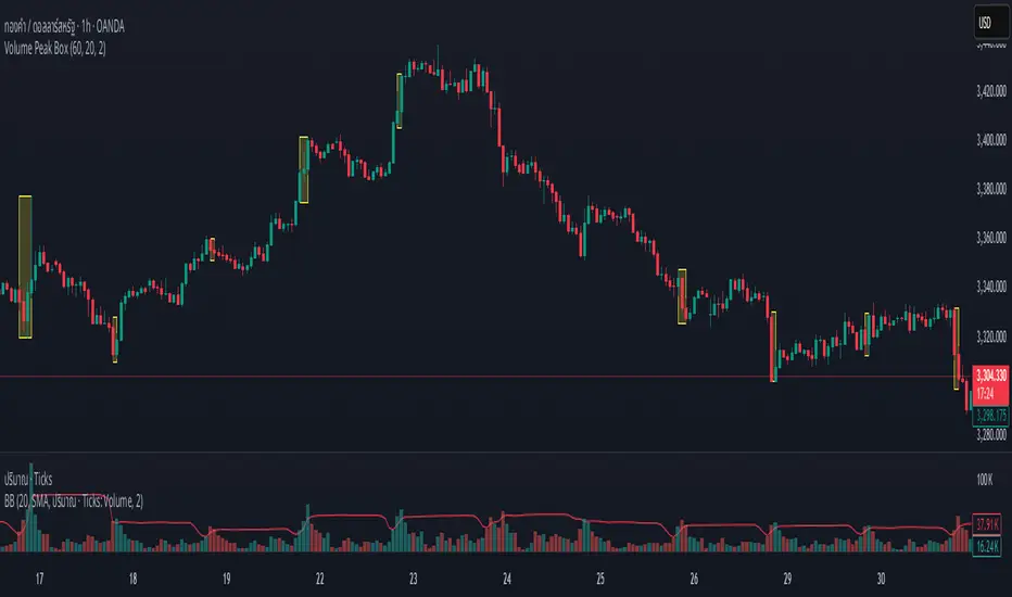
Volume Peak BoxTH Description
Volume Peak Box
อินดิเคเตอร์นี้ใช้ตรวจจับช่วงที่มี Volume สูงผิดปกติ โดยใช้ Bollinger Band กับข้อมูล Volume ที่ดึงจาก Timeframe ที่ล็อกไว้ (เช่น 1 ชั่วโมง) และจะแสดงผลในรูปแบบ กล่องครอบช่วงราคาสูง–ต่ำ ของช่วง Volume Peak นั้น
🔧 วิธีทำงาน:
คำนวณ Bollinger Band จาก Volume ของ Timeframe ที่กำหนด
ถ้า Volume สูงกว่า Upper Band → ถือว่าเป็น Volume Peak
วาดกล่องครอบ High–Low ของแท่งที่อยู่ในช่วง Volume Peak
กล่องจะแสดงบนทุก Timeframe แต่ใช้ข้อมูลจาก Timeframe ที่ล็อกไว้เท่านั้น
🧠 เหมาะสำหรับการดู:
โซน Breakout
การเคลื่อนไหวของสถาบัน
ความไม่สมดุลของอุปสงค์/อุปทาน
เหมาะมากหากใช้ร่วมกับการอ่านพฤติกรรมราคาใน Timeframe ย่อย เพื่อดูปฏิกิริยาราคาต่อแรง Volume จาก Timeframe ใหญ่
________________
ENG Description
Volume Peak Box
This indicator detects volume spikes based on Bollinger Bands applied to volume from a locked timeframe (e.g. 1H), and draws a box around the price range during those peak periods.
🔧 How it works:
Calculates Bollinger Bands on volume from the selected timeframe.
If volume exceeds the upper band, it is marked as a volume peak.
When a volume peak starts and ends, the indicator draws a box covering the high–low price range during that period.
These boxes remain visible on all timeframes, but always reflect data from the locked timeframe.
🧠 Great for identifying:
Breakout zones
Institutional activity
Supply/demand imbalances
Tip: Use with lower timeframe price action to see how the market reacts near volume peaks from higher timeframes.
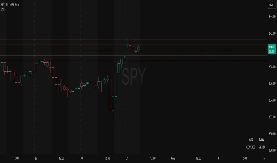
ATR Plots + OverlayATR Plots + Overlay
This tool calculates and displays Average True Range (ATR)-based levels on your chart for any selected timeframe, giving traders a quick visual reference for expected price movement relative to the most recent bar’s open price. It plots guide levels above and below that open and shows how much of the typical ATR-based range has already been covered—all in one interactive table and on-chart overlay.
What It Does
ATR Calculation:
Uses true range data over a user-defined period (default 14), smoothed via RMA, SMA, EMA, or WMA, on the selected timeframe (e.g., 1h, 4h, daily) to calculate the ATR value.
Projected Levels:
Plots four reference levels relative to the open price of the most recent bar on the chosen timeframe:
+100% ATR: Open + ATR
+50% ATR: Open + 50% of ATR
−50% ATR: Open − 50% of ATR
−100% ATR: Open − ATR
Coverage %:
Tracks high and low prices for the current session on the selected timeframe and calculates what percentage of the ATR has already been covered:
Coverage % = (High − Low) ÷ ATR × 100
Interactive Table:
Shows the ATR value and current coverage percentage in a customizable table overlay. Position, color scheme, borders, transparency, and an optional empty top row are all adjustable via settings.
Customization Options
Table Settings:
Position the table (top/bottom × left/right).
Customize background color, text color, border color, and thickness.
Optionally add an empty top row for spacing.
Line Settings:
Choose color, line style (solid/dotted/dashed), and width.
Lines automatically update with each new bar on the selected timeframe, anchored to that bar’s open price.
General Inputs:
ATR length (number of bars).
Smoothing method (RMA, SMA, EMA, WMA).
Timeframe selection for ATR calculations (e.g., 15m, 1h, Daily).
How to Use It for Trading
Measure Volatility: Quickly gauge the expected price movement based on ATR for any timeframe.
Identify Overextension: Use the coverage % to see how much of the expected ATR range is already consumed.
Plan Entries & Exits: Align trade targets and stops with ATR levels for more objective planning.
Visual Reference: Horizontal guide lines and table update automatically as new bars form, keeping information clear and actionable.
Ideal For
Intraday traders using ATR levels to frame trades.
Swing traders wanting ATR-based reference points for larger timeframes.
Anyone seeking a volatility-based framework for planning stops, targets, or identifying overextended conditions.
Circuit Breaker Table (NSE Style)🛡️ NSE Circuit Breaker Table – With Volatility-Based Band Support
This script displays a real-time circuit breaker table for any stock, showing the Upper and Lower circuit limits in a clean 2x2 grid. It’s especially useful for Indian traders monitoring NSE-listed stocks.
✅ Key Features:
📊 Upper & Lower Limits based on the previous day’s close
⚡ Optional ATR-based dynamic volatility band calculation
🎨 Customizable font sizes (Small / Medium / Large)
✅ Table neatly positioned on the top-right corner of your chart
🟢 Upper circuit shown in green, 🔴 lower circuit in red
Works on all NSE stocks and adapts automatically to charted symbols
⚙️ Customization Options:
Use static percentage bands (e.g., 10%)
Or enable ATR mode to reflect dynamic circuit potential based on recent volatility
This tool helps you stay aware of where a stock might get halted — useful for momentum traders, circuit breakout traders, and anyone monitoring volatility limits during intraday sessions.

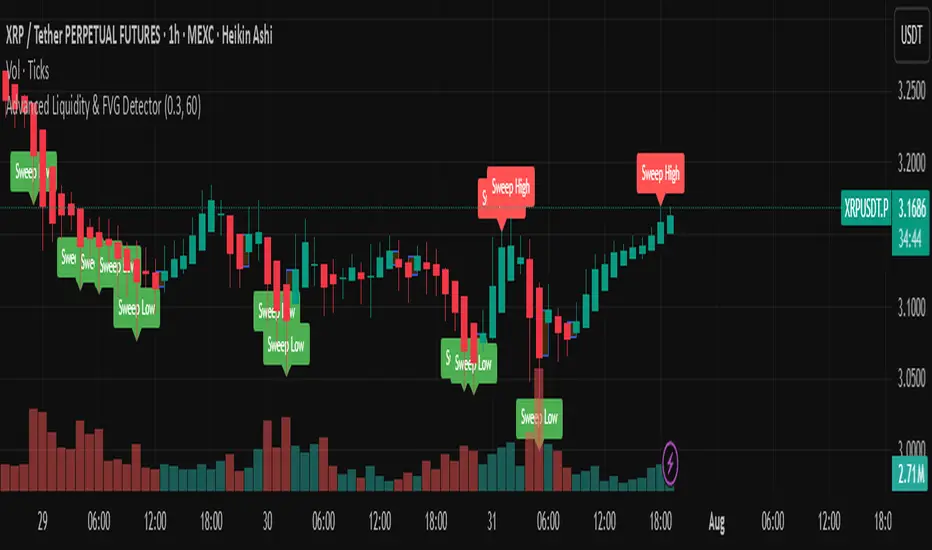
Advanced Liquidity & FVG Detector With Entry/Exit SignalsThe Advanced Liquidity & FVG Detector is more than just an indicator—it's a complete trading system that brings institutional-grade market analysis to individual traders. By combining liquidity detection, fair value gap analysis, sweep/grab pattern recognition, and intelligent risk management, this indicator provides everything needed for sophisticated market analysis and high-probability trading opportunities.
Whether you're a day trader, swing trader, or position trader, this indicator adapts to your style and timeframe, providing the insights needed to make informed trading decisions with confidence. The Pine Script v6 compatibility ensures future-proof performance and seamless integration with the latest TradingView features.
Transform your trading experience with professional-grade market structure analysis—tradable insights delivered in real-time, right on your chart.
Canonical Momenta Indicator [T1][T69]📌 Overview
The Canonical Momenta Indicator models trend pressure using a Lagrangian-based momentum engine combined with reflexivity theory to detect bursts in price movement influenced by herd behavior and volume acceleration.
🧠 Features
Lagrangian-based kinetic model combining velocity and acceleration
Reflexivity burst detection with directional scoring
Adaptive momentum-weighted output (adaptiveCMI)
Buy 🐋 / Sell 🐻 labels when reflexivity confirms direction
Fully parameterized for customization
⚙️ How to Use
This indicator helps traders:
Detect reflexive bursts in market activity driven by sharp price movement + volume spikes
Capture herd-driven directional moves early.
Gauge market pressure using a kinetic-potential energy model.
Suggested signals:
🐋 Reflexive Up: Strong bullish momentum spike confirmed by volume and positive lagrangian pressure
🐻 Reflexive Down: Strong bearish dump confirmed by volume and negative lagrangian burst
🔧 Configuration
MA Lookback Length - Smoothing for baseline price & energy calculation
Reflexivity Momentum Threshold - Price momentum trigger for burst detection
Reflexivity Lookback - Period over which bursts are counted
Reflexivity Window - Minimum burst sum to trigger signal label
Volume Spike Threshold - % above average volume to qualify as burst
📊 Behavior Description
The indicator computes a Lagrangian energy:
Kinetic Energy = (velocity² + 0.5 * acceleration²)
Potential Energy = deviation from moving average (distance²)
Lagrangian = Potential − Kinetic (higher = overextension)
Then, reflexive bursts are triggered when:
Price is rising or falling over short window (burstMvmnt)
Volume is above average by a user-defined multiple
Each bar gets a burst score:
+1 for up-burst
−1 for down-burst
0 otherwise
⚠️ Risk Profile Based on Lookback Settings
Risk Level | Description | Recommended Lookback
🟥 High | Extremely sensitive to bursts, prone to false signals | 7–10
🟨 Moderate | Balanced reflexivity with trend confirmation | 11–20
🟩 Low | Filters out most noise, slower to react | 21+
🧪 Advanced Tips
Combine with moving average slope for trend filtering
Use divergence between adaptiveCMI and price to detect exhaustion
Works well in crypto, commodities, and volatile assets
⚠️ Limitations
Sensitive to high volatility noise if volMult is too low
Designed for higher timeframes (1H, 4H, Daily) for reliability
Doesn’t confirm direction in sideways markets — pair with other filters
📝 Disclaimer
This tool is provided for educational and informational purposes. Always do your own backtesting and use proper risk management.

Smart Confluence + WinRateTwo EMAs (Fast/Slow)
Scoring Signal System (≥ 2 conditions = Buy/Sell)
Display Buy/Sell Arrows on Chart
Backtest System
Results Table: Trades, Wins, Losses, Win Rate %

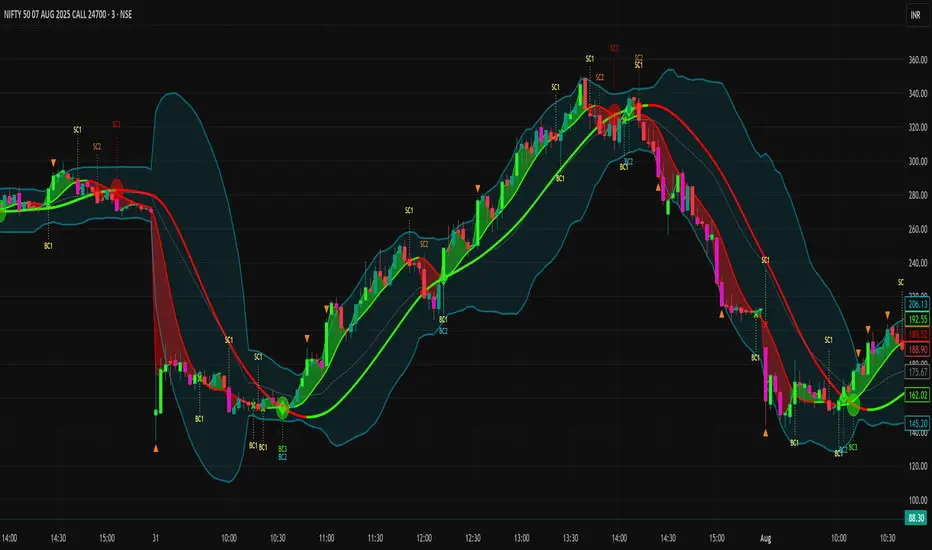
GCM Volatility-Adaptive Trend ChannelScript Description
Name: GCM Volatility-Adaptive Trend Channel (GCM VATC)
Overview
The GCM Volatility-Adaptive Trend Channel (VATC) is a comprehensive trading tool that merges the low-lag, smooth-trending capabilities of the Jurik Moving Average (JMA) with the classic volatility analysis of Bollinger Bands (BB).
By displaying both trend and volatility in a single, intuitive interface, this indicator aims to help traders see when a trend is stable versus when it's becoming volatile and might be poised for a change.
Core Components:
JMA Trend System: At its core are three dynamically colored JMA lines (Baseline, Fast, and Slow) that provide a clear view of trend direction. The lines change color based on their slope, offering immediate visual feedback on momentum. A colored ribbon between the Baseline and Fast JMA visualizes shorter-term momentum shifts.
Standard Bollinger Bands: Layered on top are standard Bollinger Bands. Calculated from the price, these bands serve as a classic measure of market volatility. They help identify periods where the market is expanding (high volatility) or contracting (low volatility).
How to Use It
By combining these two powerful concepts, this indicator provides a unified view of both trend and volatility. It can help traders to:
Identify the primary trend direction using the smooth JMA lines.
Gauge the strength and stability of that trend.
See when the market is becoming volatile (bands widening) or consolidating (bands contracting), which can often precede a significant price move or a change in trend.
A Note on Originality & House Rules Compliance
This indicator does not introduce a new mathematical formula. Instead, its strength lies in the thoughtful combination of two well-respected, publicly available concepts: the Jurik Moving Average and Bollinger Bands. The JMA implementation is a standard public version. The goal was to create a practical, all-in-one tool for trend and volatility analysis.
This script is published as fully open-source in compliance with TradingView's House Rules. It utilizes standard, publicly available algorithms and does not contain any protected or hidden code.
Settings
All lengths, sources, and colors for the JMA lines and Bollinger Bands are fully customizable in the settings menu, allowing you to tailor the indicator to your specific trading style and asset.
I hope with this indicator Traders even Beginner can can control their emotions which increase the probabilities of the winning rates and cutting the losing strength
Purposely I Didn't plant the High low or Buy Sell signals in the chart. Because everything is in the chart where volatility Signal with the Bollinger Band and Buy Sell Signal in the JMA Dynamic colors. and that's enough to decide when to take trade and when not to.
Thank You and Happy Trading
RED E Support & ResistanceThe “RED-E Support & Resistance” indicator is designed to assist traders in visualizing key levels of support and resistance on a chart by employing ATR (Average True Range) to create dynamic horizontal zones. This indicator automatically plots robust support and resistance bands that can help identify potential areas where price may reverse, consolidate, or react. These levels are particularly beneficial for traders who employ concepts like Smart Money analysis, as they illustrate zones where institutional trading activity might occur.
How It Works:
• The indicator uses ATR-based calculations to determine the placement of the support and resistance zones. This approach accounts for market volatility, making the zones adaptive to changing conditions.
• The Zone Thickness parameter allows users to customize the width of the plotted zones, enhancing visibility and fitting them to their specific trading style.
• The support and resistance zones extend horizontally across the chart, providing clear reference points for potential price reactions.
Practical Application:
• Trend Analysis: Identify areas of significant price resistance and support to understand potential turning points or trends in the market.
• Risk Management: Use these zones to better inform stop-loss placements or set profit targets.
• Confirmation Tool: Combine the indicator with other technical analysis tools for confirmation of potential trade entries or exits.
Customization Options:
• Change the colors of the support and resistance zones for better integration with different chart themes.
• Adjust the ATR Length and Multiplier to fine-tune the sensitivity of the zones based on personal preferences and the characteristics of the asset being analyzed.
Disclaimer:
This indicator is for educational and informational purposes only. It is not intended to serve as investment advice or a recommendation to buy or sell any financial instrument. Always perform your own research and consider consulting with a financial professional before making trading decisions. Trading involves significant risk, and past performance does not guarantee future results.
3 hours ago
Release Notes
The “RED-E Support & Resistance” indicator is designed to assist traders in visualizing key levels of support and resistance on a chart by employing ATR (Average True Range) to create dynamic horizontal zones. This indicator automatically plots robust support and resistance bands that can help identify potential areas where price may reverse, consolidate, or react. These levels are particularly beneficial for traders who employ concepts like Smart Money analysis, as they illustrate zones where institutional trading activity might occur.
How It Works:
• The indicator uses ATR-based calculations to determine the placement of the support and resistance zones. This approach accounts for market volatility, making the zones adaptive to changing conditions.
• The Zone Thickness parameter allows users to customize the width of the plotted zones, enhancing visibility and fitting them to their specific trading style.
• The support and resistance zones extend horizontally across the chart, providing clear reference points for potential price reactions.
Practical Application:
• Trend Analysis: Identify areas of significant price resistance and support to understand potential turning points or trends in the market.
• Risk Management: Use these zones to better inform stop-loss placements or set profit targets.
• Confirmation Tool: Combine the indicator with other technical analysis tools for confirmation of potential trade entries or exits.
Customization Options:
• Change the colors of the support and resistance zones for better integration with different chart themes.
• Adjust the ATR Length and Multiplier to fine-tune the sensitivity of the zones based on personal preferences and the characteristics of the asset being analyzed.
Disclaimer:
This indicator is for educational and informational purposes only. It is not intended to serve as investment advice or a recommendation to buy or sell any financial instrument. Always perform your own research and consider consulting with a financial professional before making trading decisions. Trading involves significant risk, and past performance does not guarantee future results.

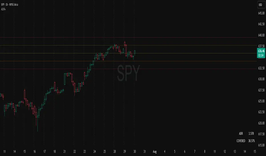
ADR Plots + OverlayADR Plots + Overlay
This tool calculates and displays Average Daily Range (ADR) levels on your chart, giving traders a quick visual reference for expected daily price movement. It plots guide levels above and below the daily open and shows how much of the day's typical range has already been covered—all in one interactive table and on-chart overlay.
What It Does
ADR Calculation:
Uses daily high-low differences over a user-defined period (default 14 days), smoothed via RMA, SMA, EMA, or WMA to calculate the average daily range.
Projected Levels:
Plots four reference levels relative to the current day's open price:
+100% ADR: Open + ADR
+50% ADR: Open + 50% of ADR
−50% ADR: Open − 50% of ADR
−100% ADR: Open − ADR
Coverage %:
Tracks intraday high and low prices to calculate what percentage of the ADR has already been covered for the current session:
Coverage % = (High − Low) ÷ ADR × 100
Interactive Table:
Shows the ADR value and today's ADR coverage percentage in a customizable table overlay. The table position, colors, border, transparency, and an optional empty top row can all be adjusted via settings.
Customization Options
Table Settings:
Position the table (top/bottom × left/right).
Change background color, text color, border color and thickness.
Toggle an empty top row for spacing.
Line Settings:
Choose color, line style (solid/dotted/dashed), and width.
Lines automatically reposition each day based on that day's open price and ADR calculation.
General Inputs:
ADR length (number of days).
Smoothing method (RMA, SMA, EMA, WMA).
How to Use It for Trading
Measure Daily Movement: Instantly know the expected daily price range based on historical volatility.
Identify Overextension: Use the coverage % to see if the market has already moved close to or beyond its typical daily range.
Plan Entries & Exits: Align trade targets and stops with ADR levels for more objective intraday planning.
Visual Reference: Horizontal guide lines and table update automatically as new data comes in, helping traders stay informed without manual calculations.
Ideal For
Intraday traders tracking daily volatility limits.
Swing traders wanting a quick reference for expected price movement per day.
Anyone seeking a volatility-based framework for planning targets, stops, or identifying extended market conditions.
NQ Phantom Scalper Pro# 👻 NQ Phantom Scalper Pro
**Advanced VWAP Mean Reversion Strategy with Volume Confirmation**
## 🎯 Strategy Overview
The NQ Phantom Scalper Pro is a sophisticated mean reversion strategy designed specifically for Nasdaq 100 (NQ) futures scalping. This strategy combines Volume Weighted Average Price (VWAP) bands with intelligent volume spike detection to identify high-probability reversal opportunities during optimal market hours.
## 🔧 Key Features
### VWAP Band System
- **Dynamic VWAP Bands**: Automatically adjusting standard deviation bands based on intraday volatility
- **Multiple Band Levels**: Configurable Band #1 (entry trigger) and Band #2 (profit target reference)
- **Flexible Anchoring**: Choose from Session, Week, Month, Quarter, or Year-based VWAP calculations
### Volume Intelligence
- **Volume Spike Detection**: Only triggers entries when volume exceeds SMA by configurable multiplier
- **Relative Volume Display**: Real-time volume strength indicator in info panel
- **Optional Volume Filter**: Can be disabled for testing alternative setups
### Advanced Time Management
- **12-Hour Format**: User-friendly time inputs (9 AM - 4 PM default)
- **Lunch Filter**: Automatically avoids low-liquidity lunch period (12-2 PM)
- **Visual Time Zones**: Color-coded background for active/inactive periods
- **Market Hours Focus**: Optimized for peak NQ trading sessions
### Smart Risk Management
- **ATR-Based Stops**: Volatility-adjusted stop losses using Average True Range
- **Dual Exit Strategy**: VWAP mean reversion + fixed profit targets
- **Adjustable Risk-Reward**: Configurable target ratio to opposite VWAP band
- **Position Sizing**: Percentage-based equity allocation
### Optional Trend Filter
- **EMA Trend Alignment**: Optional trend filter to avoid counter-trend trades
- **Configurable Period**: Adjustable EMA length for trend determination
- **Toggle Functionality**: Enable/disable based on market conditions
## 📊 How It Works
### Entry Logic
**Long Entries**: Triggered when price touches lower VWAP band + volume spike during active hours
**Short Entries**: Triggered when price touches upper VWAP band + volume spike during active hours
### Exit Strategy
1. **VWAP Mean Reversion**: Early exit when price returns to VWAP center line
2. **Profit Target**: Fixed target based on percentage to opposite VWAP band
3. **Stop Loss**: ATR-based protective stop
### Visual Elements
- **VWAP Center Line**: Blue line showing volume-weighted fair value
- **Green Bands**: Entry trigger levels (Band #1)
- **Red Bands**: Extended levels for target reference (Band #2)
- **Orange EMA**: Trend filter line (when enabled)
- **Background Colors**: Yellow (lunch), Gray (after hours), Clear (active trading)
- **Info Panel**: Real-time metrics display
## ⚙️ Recommended Settings
### Timeframes
- **Primary**: 1-5 minute charts for scalping
- **Validation**: Test on 15-minute for swing applications
### Market Conditions
- **Best Performance**: Ranging/choppy markets with good volume
- **Trend Markets**: Enable trend filter to avoid counter-trend trades
- **High Volatility**: Increase ATR multiplier for stops
### Session Optimization
- **Pre-Market**: Generally avoided (low volume)
- **Morning Session**: 9:30 AM - 12:00 PM (high activity)
- **Lunch Period**: 12:00 PM - 2:00 PM (filtered by default)
- **Afternoon Session**: 2:00 PM - 4:00 PM (good volume)
- **After Hours**: Generally avoided (wide spreads)
## ⚠️ Risk Disclaimer
This strategy is for educational purposes only and does not constitute financial advice. Past performance does not guarantee future results. Trading futures involves substantial risk of loss and is not suitable for all investors. Users should:
- Thoroughly backtest on historical data
- Start with small position sizes
- Understand the risks of leveraged trading
- Consider transaction costs and slippage
- Never risk more than you can afford to lose
## 📈 Performance Tips
1. **Volume Threshold**: Adjust volume multiplier based on average NQ volume patterns
2. **Band Sensitivity**: Modify band multipliers for different volatility regimes
3. **Time Filters**: Customize trading hours based on your timezone and preferences
4. **Trend Alignment**: Use trend filter during strong directional markets
5. **Risk Management**: Always maintain consistent position sizing and risk parameters
**Version**: 6.0 Compatible
**Asset**: Optimized for NASDAQ 100 Futures (NQ)
**Style**: Mean Reversion Scalping
**Frequency**: High-Frequency Trading Ready

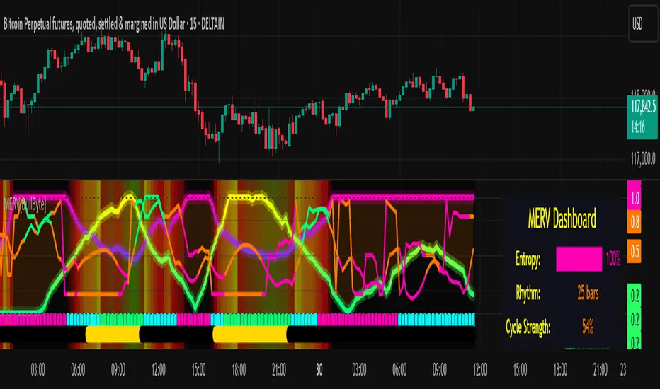
MERV: Market Entropy & Rhythm Visualizer [BullByte]The MERV (Market Entropy & Rhythm Visualizer) indicator analyzes market conditions by measuring entropy (randomness vs. trend), tradeability (volatility/momentum), and cyclical rhythm. It provides traders with an easy-to-read dashboard and oscillator to understand when markets are structured or choppy, and when trading conditions are optimal.
Purpose of the Indicator
MERV’s goal is to help traders identify different market regimes. It quantifies how structured or random recent price action is (entropy), how strong and volatile the movement is (tradeability), and whether a repeating cycle exists. By visualizing these together, MERV highlights trending vs. choppy environments and flags when conditions are favorable for entering trades. For example, a low entropy value means prices are following a clear trend line, whereas high entropy indicates a lot of noise or sideways action. The indicator’s combination of measures is original: it fuses statistical trend-fit (entropy), volatility trends (ATR and slope), and cycle analysis to give a comprehensive view of market behavior.
Why a Trader Should Use It
Traders often need to know when a market trend is reliable vs. when it is just noise. MERV helps in several ways: it shows when the market has a strong direction (low entropy, high tradeability) and when it’s ranging (high entropy). This can prevent entering trend-following strategies during choppy periods, or help catch breakouts early. The “Optimal Regime” marker (a star) highlights moments when entropy is very low and tradeability is very high, typically the best conditions for trend trades. By using MERV, a trader gains an empirical “go/no-go” signal based on price history, rather than guessing from price alone. It’s also adaptable: you can apply it to stocks, forex, crypto, etc., on any timeframe. For example, during a bullish phase of a stock, MERV will turn green (Trending Mode) and often show a star, signaling good follow-through. If the market later grinds sideways, MERV will shift to magenta (Choppy Mode), warning you that trend-following is now risky.
Why These Components Were Chosen
Market Entropy (via R²) : This measures how well recent prices fit a straight line. We compute a linear regression on the last len_entropy bars and calculate R². Entropy = 1 - R², so entropy is low when prices follow a trend (R² near 1) and high when price action is erratic (R² near 0). This single number captures trend strength vs noise.
Tradeability (ATR + Slope) : We combine two familiar measures: the Average True Range (ATR) (normalized by price) and the absolute slope of the regression line (scaled by ATR). Together they reflect how active and directional the market is. A high ATR or strong slope means big moves, making a trend more “tradeable.” We take a simple average of the normalized ATR and slope to get tradeability_raw. Then we convert it to a percentile rank over the lookback window so it’s stable between 0 and 1.
Percentile Ranks : To make entropy and tradeability values easy to interpret, we convert each to a 0–100 rank based on the past len_entropy periods. This turns raw metrics into a consistent scale. (For example, an entropy rank of 90 means current entropy is higher than 90% of recent values.) We then divide by 100 to plot them on a 0–1 scale.
Market Mode (Regime) : Based on those ranks, MERV classifies the market:
Trending (Green) : Low entropy rank (<40%) and high tradeability rank (>60%). This means the market is structurally trending with high activity.
Choppy (Magenta) : High entropy rank (>60%) and low tradeability rank (<40%). This is a mostly random, low-momentum market.
Neutral (Cyan) : All other cases. This covers mixed regimes not strongly trending or choppy.
The mode is shown as a colored bar at the bottom: green for trending, magenta for choppy, cyan for neutral.
Optimal Regime Signal : Separately, we mark an “optimal” condition when entropy_norm < 0.3 and tradeability > 0.7 (both normalized 0–1). When this is true, a ★ star appears on the bottom line. This star is colored white when truly optimal, gold when only tradeability is high (but entropy not quite low enough), and black when neither condition holds. This gives a quick visual cue for very favorable conditions.
What Makes MERV Stand Out
Holistic View : Unlike a single-oscillator, MERV combines trend, volatility, and cycle analysis in one tool. This multi-faceted approach is unique.
Visual Dashboard : The fixed on-chart dashboard (shown at your chosen corner) summarizes all metrics in bar/gauge form. Even a non-technical user can glance at it: more “█” blocks = a higher value, colors match the plots. This is more intuitive than raw numbers.
Adaptive Thresholds : Using percentile ranks means MERV auto-adjusts to each market’s character, rather than requiring fixed thresholds.
Cycle Insight : The rhythm plot adds information rarely found in indicators – it shows if there’s a repeating cycle (and its period in bars) and how strong it is. This can hint at natural bounce or reversal intervals.
Modern Look : The neon color scheme and glow effects make the lines easy to distinguish (blue/pink for entropy, green/orange for tradeability, etc.) and the filled area between them highlights when one dominates the other.
Recommended Timeframes
MERV can be applied to any timeframe, but it will be more reliable on higher timeframes. The default len_entropy = 50 and len_rhythm = 30 mean we use 30–50 bars of history, so on a daily chart that’s ~2–3 months of data; on a 1-hour chart it’s about 2–3 days. In practice:
Swing/Position traders might prefer Daily or 4H charts, where the calculations smooth out small noise. Entropy and cycles are more meaningful on longer trends.
Day trader s could use 15m or 1H charts if they adjust the inputs (e.g. shorter windows). This provides more sensitivity to intraday cycles.
Scalpers might find MERV too “slow” unless input lengths are set very low.
In summary, the indicator works anywhere, but the defaults are tuned for capturing medium-term trends. Users can adjust len_entropy and len_rhythm to match their chart’s volatility. The dashboard position can also be moved (top-left, bottom-right, etc.) so it doesn’t cover important chart areas.
How the Scoring/Logic Works (Step-by-Step)
Compute Entropy : A linear regression line is fit to the last len_entropy closes. We compute R² (goodness of fit). Entropy = 1 – R². So a strong straight-line trend gives low entropy; a flat/noisy set of points gives high entropy.
Compute Tradeability : We get ATR over len_entropy bars, normalize it by price (so it’s a fraction of price). We also calculate the regression slope (difference between the predicted close and last close). We scale |slope| by ATR to get a dimensionless measure. We average these (ATR% and slope%) to get tradeability_raw. This represents how big and directional price moves are.
Convert to Percentiles : Each new entropy and tradeability value is inserted into a rolling array of the last 50 values. We then compute the percentile rank of the current value in that array (0–100%) using a simple loop. This tells us where the current bar stands relative to history. We then divide by 100 to plot on .
Determine Modes and Signal : Based on these normalized metrics: if entropy < 0.4 and tradeability > 0.6 (40% and 60% thresholds), we set mode = Trending (1). If entropy > 0.6 and tradeability < 0.4, mode = Choppy (-1). Otherwise mode = Neutral (0). Separately, if entropy_norm < 0.3 and tradeability > 0.7, we set an optimal flag. These conditions trigger the colored mode bars and the star line.
Rhythm Detection : Every bar, if we have enough data, we take the last len_rhythm closes and compute the mean and standard deviation. Then for lags from 5 up to len_rhythm, we calculate a normalized autocorrelation coefficient. We track the lag that gives the maximum correlation (best match). This “best lag” divided by len_rhythm is plotted (a value between 0 and 1). Its color changes with the correlation strength. We also smooth the best correlation value over 5 bars to plot as “Cycle Strength” (also 0 to 1). This shows if there is a consistent cycle length in recent price action.
Heatmap (Optional) : The background color behind the oscillator panel can change with entropy. If “Neon Rainbow” style is on, low entropy is blue and high entropy is pink (via a custom color function), otherwise a classic green-to-red gradient can be used. This visually reinforces the entropy value.
Volume Regime (Dashboard Only) : We compute vol_norm = volume / sma(volume, len_entropy). If this is above 1.5, it’s considered high volume (neon orange); below 0.7 is low (blue); otherwise normal (green). The dashboard shows this as a bar gauge and percentage. This is for context only.
Oscillator Plot – How to Read It
The main panel (oscillator) has multiple colored lines on a 0–1 vertical scale, with horizontal markers at 0.2 (Low), 0.5 (Mid), and 0.8 (High). Here’s each element:
Entropy Line (Blue→Pink) : This line (and its glow) shows normalized entropy (0 = very low, 1 = very high). It is blue/green when entropy is low (strong trend) and pink/purple when entropy is high (choppy). A value near 0.0 (below 0.2 line) indicates a very well-defined trend. A value near 1.0 (above 0.8 line) means the market is very random. Watch for it dipping near 0: that suggests a strong trend has formed.
Tradeability Line (Green→Yellow) : This represents normalized tradeability. It is colored bright green when tradeability is low, transitioning to yellow as tradeability increases. Higher values (approaching 1) mean big moves and strong slopes. Typically in a market rally or crash, this line will rise. A crossing above ~0.7 often coincides with good trend strength.
Filled Area (Orange Shade) : The orange-ish fill between the entropy and tradeability lines highlights when one dominates the other. If the area is large, the two metrics diverge; if small, they are similar. This is mostly aesthetic but can catch the eye when the lines cross over or remain close.
Rhythm (Cycle) Line : This is plotted as (best_lag / len_rhythm). It indicates the relative period of the strongest cycle. For example, a value of 0.5 means the strongest cycle was about half the window length. The line’s color (green, orange, or pink) reflects how strong that cycle is (green = strong). If no clear cycle is found, this line may be flat or near zero.
Cycle Strength Line : Plotted on the same scale, this shows the autocorrelation strength (0–1). A high value (e.g. above 0.7, shown in green) means the cycle is very pronounced. Low values (pink) mean any cycle is weak and unreliable.
Mode Bars (Bottom) : Below the main oscillator, thick colored bars appear: a green bar means Trending Mode, magenta means Choppy Mode, and cyan means Neutral. These bars all have a fixed height (–0.1) and make it very easy to see the current regime.
Optimal Regime Line (Bottom) : Just below the mode bars is a thick horizontal line at –0.18. Its color indicates regime quality: White (★) means “Optimal Regime” (very low entropy and high tradeability). Gold (★) means not quite optimal (high tradeability but entropy not low enough). Black means neither condition. This star line quickly tells you when conditions are ideal (white star) or simply good (gold star).
Horizontal Guides : The dotted lines at 0.2 (Low), 0.5 (Mid), and 0.8 (High) serve as reference lines. For example, an entropy or tradeability reading above 0.8 is “High,” and below 0.2 is “Low,” as labeled on the chart. These help you gauge values at a glance.
Dashboard (Fixed Corner Panel)
MERV also includes a compact table (dashboard) that can be positioned in any corner. It summarizes key values each bar. Here is how to read its rows:
Entropy : Shows a bar of blocks (█ and ░). More █ blocks = higher entropy. It also gives a percentage (rounded). A full bar (10 blocks) with a high % means very chaotic market. The text is colored similarly (blue-green for low, pink for high).
Rhythm : Shows the best cycle period in bars (e.g. “15 bars”). If no calculation yet, it shows “n/a.” The text color matches the rhythm line.
Cycle Strength : Gives the cycle correlation as a percentage (smoothed, as shown on chart). Higher % (green) means a strong cycle.
Tradeability : Displays a 10-block gauge for tradeability. More blocks = more tradeable market. It also shows “gauge” text colored green→yellow accordingly.
Market Mode : Simply shows “Trending”, “Choppy”, or “Neutral” (cyan text) to match the mode bar color.
Volume Regime : Similar to tradeability, shows blocks for current volume vs. average. Above-average volume gives orange blocks, below-average gives blue blocks. A % value indicates current volume relative to average. This row helps see if volume is abnormally high or low.
Optimal Status (Large Row) : In bold, either “★ Optimal Regime” (white text) if the star condition is met, “★ High Tradeability” (gold text) if tradeability alone is high, or “— Not Optimal” (gray text) otherwise. This large row catches your eye when conditions are ripe.
In short, the dashboard turns the numeric state into an easy read: filled bars, colors, and text let you see current conditions without reading the plot. For instance, five blue blocks under Entropy and “25%” tells you entropy is low (good), and a row showing “Trending” in green confirms a trend state.
Real-Life Example
Example : Consider a daily chart of a trending stock (e.g. “AAPL, 1D”). During a strong uptrend, recent prices fit a clear upward line, so Entropy would be low (blue line near bottom, perhaps below the 0.2 line). Volatility and slope are high, so Tradeability is high (green-yellow line near top). In the dashboard, Entropy might show only 1–2 blocks (e.g. 10%) and Tradeability nearly full (e.g. 90%). The Market Mode bar turns green (Trending), and you might see a white ★ on the optimal line if conditions are very good. The Volume row might light orange if volume is above average during the rally. In contrast, imagine the same stock later in a tight range: Entropy will rise (pink line up, more blocks in dashboard), Tradeability falls (fewer blocks), and the Mode bar turns magenta (Choppy). No star appears in that case.
Consolidated Use Case : Suppose on XYZ stock the dashboard reads “Entropy: █░░░░░░░░ 20%”, “Tradeability: ██████████ 80%”, Mode = Trending (green), and “★ Optimal Regime.” This tells the trader that the market is in a strong, low-noise trend, and it might be a good time to follow the trend (with appropriate risk controls). If instead it reads “Entropy: ████████░░ 80%”, “Tradeability: ███▒▒▒▒▒▒ 30%”, Mode = Choppy (magenta), the trader knows the market is random and low-momentum—likely best to sit out until conditions improve.
Example: How It Looks in Action
Screenshot 1: Trending Market with High Tradeability (SOLUSD, 30m)
What it means:
The market is in a clear, strong trend with excellent conditions for trading. Both trend-following and active strategies are favored, supported by high tradeability and strong volume.
Screenshot 2: Optimal Regime, Strong Trend (ETHUSD, 1h)
What it means:
This is an ideal environment for trend trading. The market is highly organized, tradeability is excellent, and volume supports the move. This is when the indicator signals the highest probability for success.
Screenshot 3: Choppy Market with High Volume (BTC Perpetual, 5m)
What it means:
The market is highly random and choppy, despite a surge in volume. This is a high-risk, low-reward environment, avoid trend strategies, and be cautious even with mean-reversion or scalping.
Settings and Inputs
The script is fully open-source; here are key inputs the user can adjust:
Entropy Window (len_entropy) : Number of bars used for entropy and tradeability (default 50). Larger = smoother, more lag; smaller = more sensitivity.
Rhythm Window (len_rhythm ): Bars used for cycle detection (default 30). This limits the longest cycle we detect.
Dashboard Position : Choose any corner (Top Right default) so it doesn’t cover chart action.
Show Heatmap : Toggles the entropy background coloring on/off.
Heatmap Style : “Neon Rainbow” (colorful) or “Classic” (green→red).
Show Mode Bar : Turn the bottom mode bar on/off.
Show Dashboard : Turn the fixed table panel on/off.
Each setting has a tooltip explaining its effect. In the description we will mention typical settings (e.g. default window sizes) and that the user can move the dashboard corner as desired.
Oscillator Interpretation (Recap)
Lines : Blue/Pink = Entropy (low=trend, high=chop); Green/Yellow = Tradeability (low=quiet, high=volatile).
Fill : Orange tinted area between them (for visual emphasis).
Bars : Green=Trending, Magenta=Choppy, Cyan=Neutral (at bottom).
Star Line : White star = ideal conditions, Gold = good but not ideal.
Horizontal Guides : 0.2 and 0.8 lines mark low/high thresholds for each metric.
Using the chart, a coder or trader can see exactly what each output represents and make decisions accordingly.
Disclaimer
This indicator is provided as-is for educational and analytical purposes only. It does not guarantee any particular trading outcome. Past market patterns may not repeat in the future. Users should apply their own judgment and risk management; do not rely solely on this tool for trading decisions. Remember, TradingView scripts are tools for market analysis, not personalized financial advice. We encourage users to test and combine MERV with other analysis and to trade responsibly.
-BullByte
HMM Trend Strength Meter (3-State)Strong Up-Trend: p_up > 0.6–0.7 → look for BUY setups
Strong Down-Trend: p_dn > 0.6–0.7 → look for SELL setups
Range/Sideways: p_side > 0.6 → consider mean-reversion entries
Adjust your own threshold (e.g. 0.7–0.8) to control signal frequency.
VWAP MultiCombined IntradayIncluded all VWAP in One for intraday purpose.
User will get S W M Q Y Decade Century Vwap at Single Combined.
This will helps to find levels who uses vwap on routine basis.
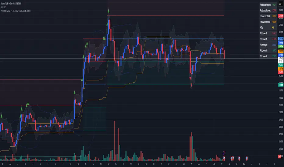
Combined Predictive Indicator### Combined Predictive Zones & Levels
This indicator is a powerful hybrid tool designed to provide a comprehensive map of potential future price action. It merges two distinct predictive models into a single, cohesive view, helping traders identify key levels of support, resistance, and areas of high confluence.
#### How It Works: Two Models in One
This script is built on two core components that you can use together or analyze separately:
**Part 1: Classic Range & Fibonacci Prediction**
This model uses classic technical analysis principles to project a potential range for the upcoming price action.
* **Highest High / Lowest Low:** It identifies the significant trading range over a user-defined lookback period.
* **Fibonacci Levels:** It automatically plots key Fibonacci retracement levels (e.g., 38.2% and 61.8%) within this range, which often act as critical support or resistance.
* **ATR & Average Range:** It calculates a "predicted" upper and lower boundary based on the average historical range and current volatility (ATR).
**Part 2: Advanced Predictive Ranges (Self-Adjusting Channels)**
This is a dynamic model that creates adaptive support and resistance zones based on a smoothed average price and volatility.
* **Dynamic Average:** It uses a unique moving average that only adjusts when the price moves significantly, creating a stable baseline.
* **ATR-Based Zones:** It projects multiple levels of support (S1, S2) and resistance (R1, R2) around this average, which widen and narrow based on market volatility. These zones often signal areas where price might stall or reverse.
#### Key Features:
* **Hybrid Model for Confluence:** The true power of this indicator lies in finding where the levels from both models overlap. A Fibonacci level aligning with a Predictive Range support zone is a much stronger signal.
* **Comprehensive Data Table:** A clean, on-chart table displays the precise values of all key predictive levels, allowing for quick reference and precise trade planning.
* **Multi-Timeframe (MTF) Capability:** The Advanced Predictive Ranges can be calculated on a higher timeframe, giving you a broader market context.
* **Fully Customizable:** All lengths, multipliers, and levels for both models are fully adjustable in the settings to fit any asset or trading style.
* **Clear Visuals:** All zones and levels are color-coded for intuitive and easy-to-read analysis.
#### How to Use:
1. Look for areas of **confluence** where multiple levels from both models cluster together. These are high-probability zones for price reactions.
2. Use the Predictive Range zones (S1/S2 and R1/R2) as potential targets for trades or as areas to watch for entries and exits.
3. Pay attention to the on-chart table for exact price levels to set limit orders or stop-losses.
**Disclaimer:** This script is an analytical tool for educational purposes and should not be considered financial advice. All trading involves risk. Past performance is not indicative of future results. Always use this indicator as part of a comprehensive trading strategy with proper risk management.
Feedback is welcome! If you find this tool useful, please leave a like.
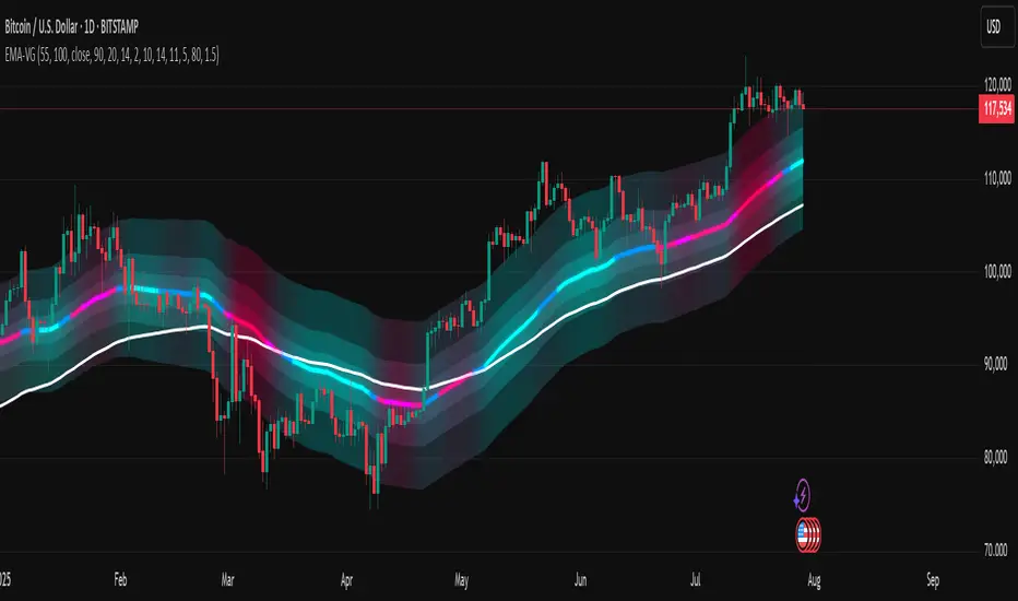
[LeonidasCrypto]EMA with Volatility GlowEMA Volatility Glow - Advanced Moving Average with Dynamic Volatility Visualization
Overview
The EMA Volatility Glow indicator combines dual exponential moving averages with a sophisticated volatility measurement system, enhanced by dynamic visual effects that respond to real-time market conditions.
Technical Components
Volatility Calculation Engine
BB Volatility Curve: Utilizes Bollinger Band width normalized through RSI smoothing
Multi-stage Noise Filtering: 3-layer exponential smoothing algorithm reduces market noise
Rate of Change Analysis: Dual-timeframe RoC calculation (14/11 periods) processed through weighted moving average
Dynamic Normalization: 100-period lookback for relative volatility assessment
Moving Average System
Primary EMA: Default 55-period exponential moving average with volatility-responsive coloring
Secondary EMA: Default 100-period exponential moving average for trend confirmation
Trend Analysis: Real-time bullish/bearish determination based on EMA crossover dynamics
Visual Enhancement Framework
Gradient Band System: Multi-layer volatility bands using Fibonacci ratios (0.236, 0.382, 0.618)
Dynamic Color Mapping: Five-tier color system reflecting volatility intensity levels
Configurable Glow Effects: Customizable transparency and intensity settings
Trend Fill Visualization: Directional bias indication between moving averages
Key Features
Volatility States:
Ultra-Low: Minimal market movement periods
Low: Reduced volatility environments
Medium: Normal market conditions
High: Increased volatility phases
Extreme: Exceptional market stress periods
Customization Options:
Adjustable EMA periods
Configurable glow intensity (1-10 levels)
Variable transparency controls
Toggleable visual components
Customizable gradient band width
Technical Calculations:
ATR-based gradient bands with noise filtering
ChartPrime-inspired multi-layer fill system
Real-time volatility curve computation
Smooth color gradient transitions
Applications
Trend Identification: Dual EMA system for directional bias assessment
Volatility Analysis: Real-time market stress evaluation
Risk Management: Visual volatility cues for position sizing decisions
Market Timing: Enhanced visual feedback for entry/exit consideration
Daily ATR Stop Loss Buffer- Calculates Daily ATR: Uses the daily timeframe ATR (Average True Range) - a measure of price volatility
- Applies Your Buffer: Takes a percentage of that ATR that you set in the settings (e.g., 5% of daily ATR)
- Creates Stop Levels: Calculates where to place stop losses based on current price plus/minus your ATR buffer

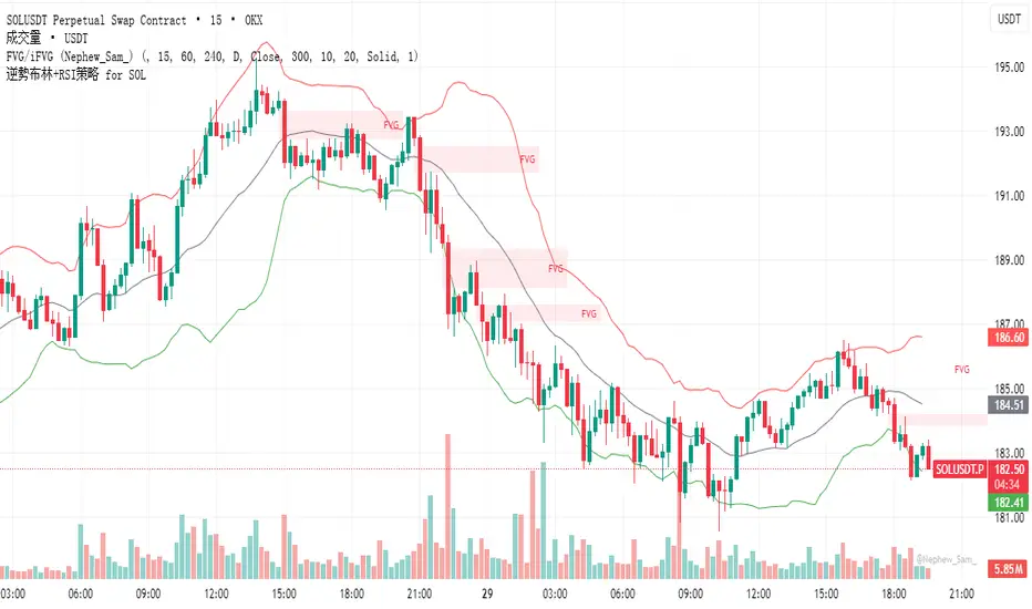
逆勢布林+RSI策略 for SOL可以直接套用到 SOLUSDT, SOLPERP, 或其他 SOL 合約。
在策略回測介面中選擇 5min 或 15min 看策略表現。
若要調整停利%或 RSI 數值,改變 rsi < 25 與 (shortEntryPrice - close) / shortEntryPrice >= 0.035 即可。
This can be directly applied to SOLUSDT, SOLPERP, or other SOL futures.
In the strategy backtesting interface, select 5-minute or 15-minute periods to view strategy performance.
To adjust the take-profit percentage or RSI value, set RSI < 25 and (shortEntryPrice - close) / shortEntryPrice >= 0.035.
Anti Nyangkut – Indikator Karya Anak Bangsa Anti Nyangkut – Indikator Karya Anak Bangsa
Indikator ini khusus buat kamu yang sering beli di pucuk dan jual di support, lalu akhirnya jadi bahan backtest orang lain.
💡 Sinyal buy only - muncul kalau harga udah:
✅ Di atas MA5
✅ Di atas Bollinger Bands Upper
✅ Di atas VWAP (khusus 1H & 4H)
🟢 TP dan SL otomatis muncul — biar gak cuma "niat hold sampe hijau"
📊 Cocok buat scalping & swing di 1H / 4H / 1D
Gak ada sinyal jual. Exit di tangan masing-nasing, jangan lupa pasang SL.
—
100% gratis. Bayarnya pakai amal jariyah.
—
Anti Nyangkut – An Indicator by the People, for the People
This one's for you if you always buy the top, sell the bottom, and end up becoming someone else's backtest data.
💡 Buy-Only Signals — triggered when price is:
✅ Above MA5
✅ Above Bollinger Bands Upper
✅ Above VWAP (on 1H & 4H only)
🟢 Auto TP & SL lines — so you stop saying "I'll hold until it turns green"
📊 Perfect for scalping & swing trades on 1H / 4H / 1D
There’s no sell signal. Exits are your responsibility — just don’t skip the stop loss.
—
100% free. Just pay with good karma.

VIX9D to VIX RatioVIX9D to VIX Ratio
The ratio > 1 can signal near-term fear > long-term fear (potential short-term stress).
The ratio < 1 implies long-term implied volatility is higher — more typical in calm markets.

ADR Tracker Version 2Description
The **ADR Tracker** plots a customizable panel on your chart that monitors the Average Daily Range (ADR) and shows how today’s price action compares to that average. It calculates the daily high–low range for each of the past 14 days (can be adjusted) and then takes a simple moving average of those ranges to determine the ADR.
**Features:**
* **Current ADR value:** Shows the 14‑day ADR in price units.
* **ADR status:** Indicates whether today’s range has reached or exceeded the ADR.
* **Ticks remaining:** Calculates how many minimum price ticks remain before the ADR would be met.
* **Real‑time tracking:** Monitors the intraday high and low to update the range continuously.
* **Customizable panel:** Uses TradingView’s table object to display the information. You can set the table’s horizontal and vertical position (top/middle/bottom and left/centre/right) with inputs. The script also lets you change the text and background colours, as well as the width and height of each row. Table cells use explicit width and height percentages, which Pine supports in v6. Each call to `table.cell()` defines the text, colours and dimensions for its cell, so the panel resizes automatically based on your settings.
**Usage:**
Apply the indicator to any chart. For the most accurate real‑time tracking, use it on intraday timeframes (e.g. 5‑min or 1‑hour) so the current day’s range updates as new bars arrive. Adjust the inputs in the settings panel to reposition the list or change its appearance.
---
This description explains what the indicator does and highlights its customizable table display, referencing the Pine Script table features used.
