Global Liquidity Indicator in USDThis indicator aggregates the total central bank balance sheets and M2 money supply for the USA, Canada, China, European Union, Japan, and the UK, converting all values to USD and normalizing them to trillions for easy visualization. It plots three lines: Total Balance Sheet, Total M2, and Combined Total, providing a comprehensive view of global liquidity trends.
Key Features:
Dynamic Coloring: Customize line colors based on direction—green for upward trends, red for downward (or any colors you choose), with independent on/off toggles for each line.
Real-Time Currency Conversion: Uses live forex rates (e.g., USD/CNY, USD/EUR) for accurate USD conversions.
Statistics

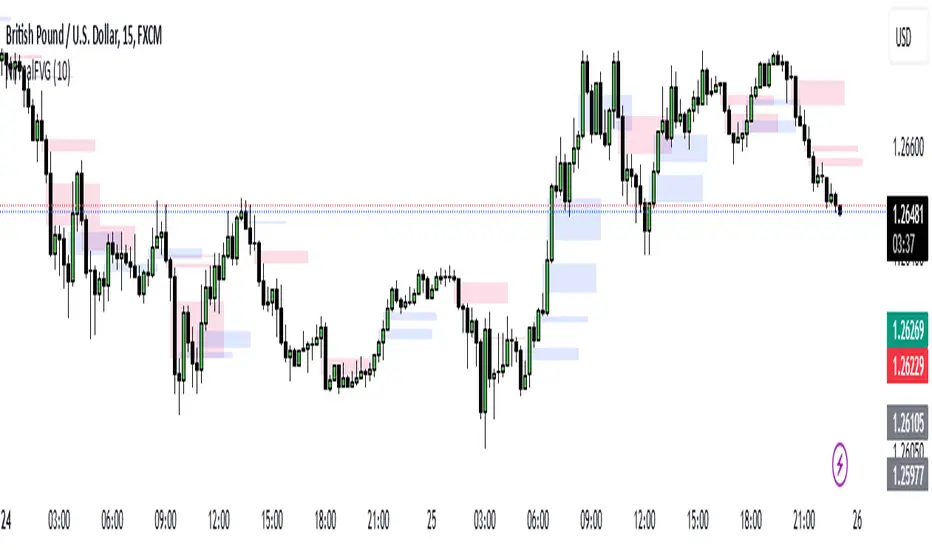
Nirmal Fair Value GapsICT Fair Value Gaps
Trade Wisely
How a Fair Value Gap Works
Formation:
A Fair Value Gap occurs when a strong price movement (usually from institutional orders) creates an imbalance between buyers and sellers.
This is typically seen in a three-candle pattern, where the middle candle has a large body, and the two surrounding candles have wicks but little overlap with the middle candle’s range.
Identification:
The FVG is marked between the high of the first candle and the low of the third candle (for bullish gaps).
For bearish gaps, it’s the low of the first candle and the high of the third candle.
Market Behavior Around FVG:
Price often retraces into the gap before resuming its original direction.
This happens because the market seeks to "fill" the imbalance where few trades occurred.
Traders use FVGs as potential entry zones for trend continuation trades.
Trading Fair Value Gaps
In an Uptrend:
Look for bullish fair value gaps as potential support zones for buy entries.
Price may dip into the gap and then continue upward.
In a Downtrend:
Look for bearish fair value gaps as potential resistance zones for sell entries.
Price may retrace into the gap and then drop further.
Confluence Factors:
FVGs work best when combined with other strategies like order blocks, liquidity zones, or key Fibonacci levels.
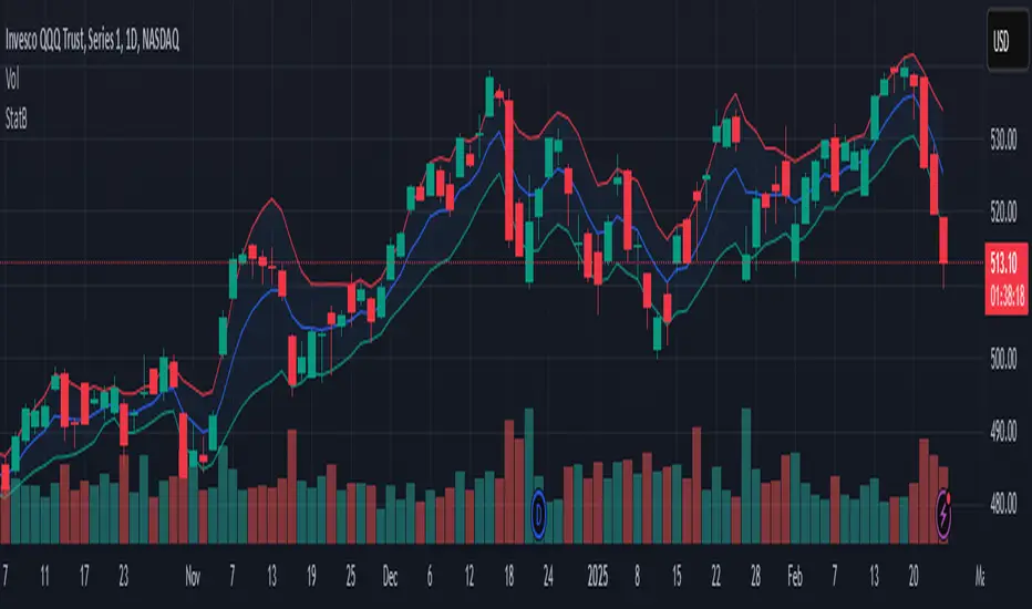
Statistical BandsThis TradingView indicator, "Statistical Bands" (short title "StatB"), creates a dynamic envelope around a smoothed baseline by combining noise reduction techniques with volatility measurement. It offers several smoothing methods—including various moving averages and a Kalman filter option—and calculates upper and lower bands based on either standard deviation or ATR, allowing traders to visualize potential support/resistance and volatility levels.
Overview
Baseline Calculation:
The indicator computes a baseline from a user-selected source (typically the close price) and smooths it using a chosen algorithm. If the user selects “Kalman,” the script applies a Kalman filter (using user-defined parameters for measurement noise variance (R) and process noise variance (Q)); otherwise, it uses one of several moving averages (SMA, EMA, RMA, WMA, VWMA, or HMA).
Band Formation:
A statistical measure of volatility—either the standard deviation or the Average True Range (ATR)—is calculated over a specified length and then multiplied by a user-defined bandwidth multiplier. The upper and lower bands are obtained by adding or subtracting this value from the baseline.
Visualization:
The indicator plots the baseline and the two bands over the price chart and fills the area between the bands with a semi-transparent color, making it easier to identify potential breakout zones or areas of support and resistance.
This concise yet flexible tool aids traders in assessing current market conditions by highlighting volatility and potential turning points.
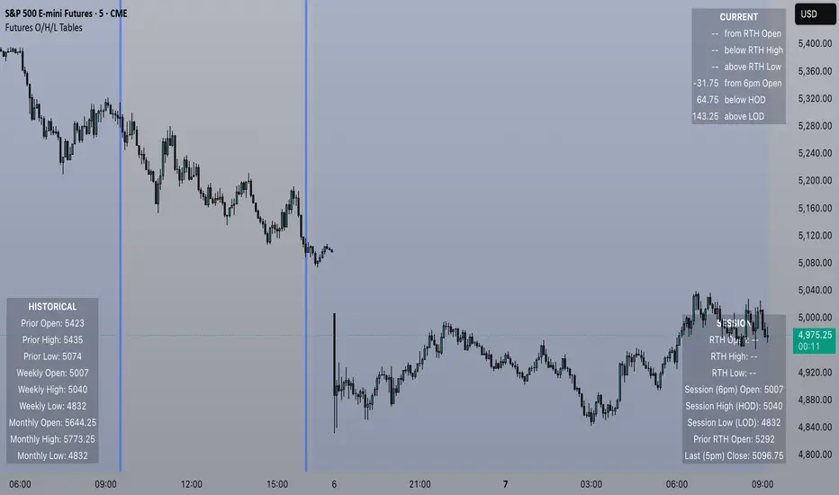
Futures Open/High/Low TablesAdds (up to) 3 tables to a chart, displaying Open/High/Low data for today (RTH and extended hours), yesterday, and the current week / month -- to help with intraday analysis of a futures ticker.
The tables only appear on intraday charts (5min, 30min, etc). On a Daily/Weekly/etc chart they are not calculated or shown.
In addition to Open/High/Low, the "Current" table in the top-right shows a live measurement of # of points from the open, the RTH open, and the highs/lows.
Lastly, the 9:30am ET open and the 4pm RTH close are by default marked with a shaded background (on intraday charts) for easy visual reference, and also to help with adjusting the session time to accommodate time zone issues if they occur.
Tested on ES in Eastern Time Zone, but should work on any futures instrument and any time zone by adjusting the Session Time setting.
Celestial Pair Spread Hello friends, after a very long time!
Today, I tried to put into code an idea that came to my mind spontaneously and suddenly.
Note :
This script is experimental and improvable.
I haven't had a chance to try it yet.
TIMEFRAME : 1D (Daily Bars)
CELESTIAL SPREAD
The spread moves in a very limited area and is consistent within itself, especially on days far from the end of the contract.
That's why there is a reassuring sky atmosphere. That's why this name was given completely improvised.
Basic logic of the script
We enter the name of the CME Futures contract we want to enter:
Ex : CL1! , ES1! , ZC1! , NQ1!
The script creates us a pair trade parity divided into secondary contracts.
Example : ES1!/ES2!
What is pair trading?
I will explain briefly here.
For users who are wondering:
www.investopedia.com
Let's get back to our topic.
Now we have created a parity that does not actually exist.
This parity is the manifestation of the relative movements of two contracts.
When the parity rises, ES1! increased,ES2! has fallen.
In the opposite case, We can say: ES1! Contract has been dropped ES2! has increased.
Pair trading is generally a trade that needs to be kept in mind from time to time.
It is a method preferred by professionals who can process very quickly.
Market risk is minimal, but since 2 contracts are purchased, more money is paid and very low percentage profits are made.
It is very expensive to do pair trading, especially with oil and its derivatives and interest security derivatives.
The contract we are considering has micros. (small-item contracts tied to the same value)
So when we switch to our broker MES1!/MES2! We will trade.
For all CME futures :
www.cmegroup.com
Anyway, let's continue:
The script created the parity showing its relationship with the next contract and plotted it as bars.
Celestial bands are just like Bollinger bands, but they consist of 3 bands based on percentage changes rather than standard deviation.
The middle band is obtained from moving averages.
The upper and lower bands are the middle band subjected to a threshold value.
The threshold value can be changed.
0.15 percent was charged for this script.
CAUTION :
As can be seen in the example below;
The most important thing is not to make any transactions when the contract switch dates are approaching.
Therefore, it is recommended to use it just below the main chart.
The blue bars in the parity are
Values that outside the upper and lower threshold values are colored blue.
For this condition
Alerts has been added.
Don't forget to add alert and edit.
MAIN PURPOSE
It is aimed to start a pair trade when such conditions come and to quickly close the trades when the parity basis reaches the value.
OTHER IMPORTANT POINTS
Other issues are broker related issues.
Difference between initial margins and maintanence margins of contracts (between 1! and 2!)
It shouldn't be too high.
The commission should not be too high.
Leverage must be high because the profit percentage is very low.
To calculate leverage you must divide your contract size by the relevant margin requirement.
Sample margin requirement table:
www.interactivebrokers.com
RISKS
It is an experimental and intellectual script,
the risk of contract price differences (maybe it will not leave a profit except for very extreme values)
I remind you of the quickness risk that comes from a two-legged trade.
Alerts definitely synchronized with an audible alert sent to a smartphone as an e-mail notification and displayed on the locked screen for quick action.
Best regards!

DCSessionStatsOHLC_v1.0DCSessionStatsOHLC_v1.0
© dc_77 | Pine Script™ v6 | Licensed under Mozilla Public License 2.0
This indicator overlays customizable session-based OHLC (Open, High, Low, Close) statistics on your TradingView chart. It tracks price action within user-defined sessions, calculates average manipulation and distribution levels based on historical data, and visually projects these levels with lines and labels. Additionally, it provides a session count table to monitor bullish and bearish sessions.
Key Features:
Session Customization: Define session time (e.g., "0000-1600") and time zone (e.g., UTC, America/New_York). Analyze up to 20 historical sessions.
Anchor Line: Displays a vertical line at session start with customizable style, color, and optional label.
Session Open Line: Plots a horizontal line at the session’s opening price with adjustable appearance and label.
Manipulation Levels: Calculates and projects average price extensions (high/low relative to open) for manipulative moves, shown as horizontal lines with labels.
Distribution Levels: Displays average price ranges (high/low beyond open) for distribution phases, with customizable lines and labels.
Visual Flexibility: Adjust line styles (solid, dashed, dotted), colors, widths, label sizes, and projection offsets (bars beyond session start).
Session Stats Table: Optional table showing counts of bullish (close > open) and bearish (close < open) sessions, with configurable position and size.
How It Works:
Tracks OHLC data within each session and identifies session start/end based on the specified time range.
Computes averages for manipulation (e.g., low below open in bullish sessions) and distribution (e.g., high above open) levels from past sessions.
Projects these levels forward as horizontal lines, extending them by a user-defined offset for easy reference.
Updates a table with real-time bullish/bearish session counts.
Use Case:
Ideal for traders analyzing intraday or custom session behavior, identifying key price levels, and gauging market sentiment over time.
Toggle individual elements on/off and fine-tune visuals to suit your trading style.

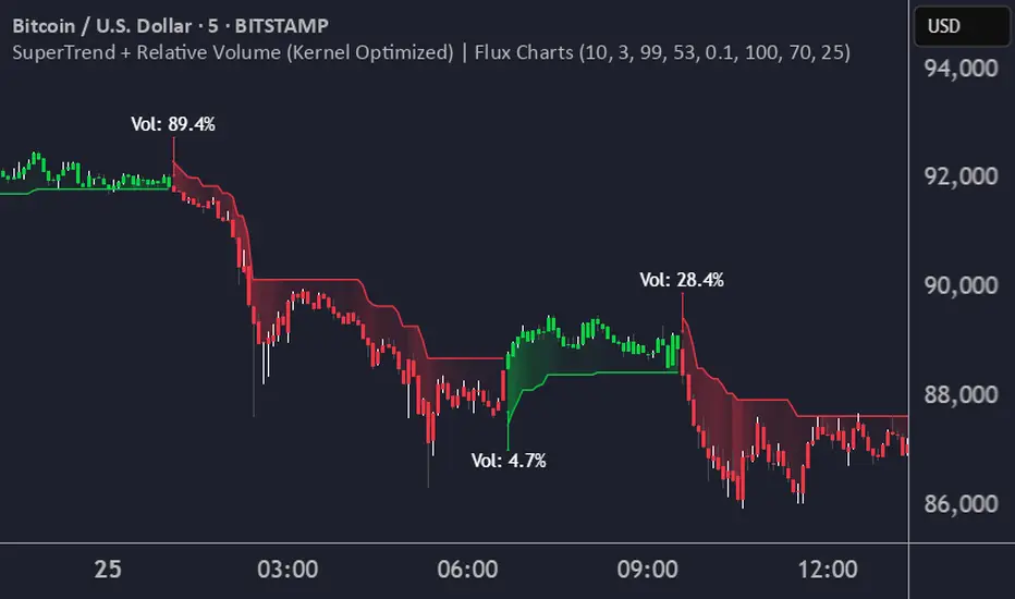
SuperTrend + Relative Volume (Kernel Optimized)Introducing our new KDE Optimized Supertrend + Relative Volume Indicator!
This innovative indicator combines the power of the Supertrend indicator along with Relative Volume. It utilizes the Kernel Density Estimation (KDE) to estimate the probability of a candlestick marking a significant trend break or reversal.
❓How to Interpret the KDE %:
The KDE % is a crucial metric that reflects the likelihood that the current candlestick represents a true break in the SuperTrend line, supported by an increase in relative volume. It estimates the probability of a trend shift or continuation based on historical SuperTrend breaks and volume patterns:
Low KDE %: A lower probability that the current break is significant. Price action is less likely to reverse, and the trend may continue.
Moderate KDE - High KDE %: An increased possibility that a trend reversal or consolidation could occur. Traders should start watching for confirmation signals.
📌How Does It Work?
The SuperTrend indicator uses the Average True Range (ATR) to determine the direction of the trend and identifies when the price crosses the SuperTrend line, signaling a potential trend reversal. Here's how the KDE Optimized SuperTrend Indicator works:
SuperTrend Calculation: The SuperTrend indicator is calculated, and when the price breaks above (bullish) or below (bearish) the SuperTrend line, it is logged as a significant event.
Relative Volume: For each break in the SuperTrend line, we calculate the relative volume (current volume vs. the average volume over a defined period). High relative volume can suggest stronger confirmation of the trend break.
KDE Array Calculation: KDE is applied to the break points and relative volume data:
Define the KDE options: Bandwidth, Number of Steps, and Array Range (Array Max - Array Min).
Create a density range array using the defined number of steps, corresponding to potential break points.
Apply a Gaussian kernel function to the break points and volume data to estimate the likelihood of the trend break being significant.
KDE Value and Signal Generation: The KDE array is updated as each break occurs. The KDE % is calculated for the breakout candlestick, representing the likelihood of the trend break being significant. If the KDE value exceeds the defined activation threshold, a darker bullish or bearish arrow is plotted after bar confirmation. If the KDE value falls below the threshold, a more transparent arrow is drawn, indicating a possible but lower probability break.
⚙️Settings:
SuperTrend Settings:
ATR Length: The period over which the Average True Range (ATR) is calculated.
Multiplier: The multiplier applied to the ATR to determine the SuperTrend threshold.
KDE Settings:
Bandwidth: Determines the smoothness of the KDE function and the width of the influence of each break point.
Number of Bins (Steps): Defines the precision of the KDE algorithm, with higher values offering more detailed calculations.
KDE Threshold %: The level at which relative volume is considered significant for confirming a break.
Relative Volume Length: The number of historic candles used in calculating KDE %
DynamicMALibrary "DynamicMA"
Dynamic Moving Averages Library
Introduction
The Dynamic Moving Averages Library is a specialized collection of custom built functions designed to calculate moving averages dynamically, beginning from the first available bar. Unlike standard moving averages, which rely on fixed length lookbacks, this library ensures that indicators remain fully functional from the very first data point, making it an essential tool for analysing assets with short time series or limited historical data.
This approach allows traders and developers to build robust indicators that do not require a preset amount of historical data before generating meaningful outputs. It is particularly advantageous for:
Newly listed assets with minimal price history.
High-timeframe trading, where large lookback periods can lead to delayed or missing data.
By eliminating the constraints of fixed lookback periods, this library enables the seamless construction of trend indicators, smoothing functions, and hybrid models that adapt instantly to market conditions.
Comprehensive Set of Custom Moving Averages
The library includes a wide range of custom dynamic moving averages, each designed for specific analytical use cases:
SMA (Simple Moving Average) – The fundamental moving average, dynamically computed.
EMA (Exponential Moving Average) – Adaptive smoothing for better trend tracking.
DEMA (Double Exponential Moving Average) – Faster trend detection with reduced lag.
TEMA (Triple Exponential Moving Average) – Even more responsive than DEMA.
WMA (Weighted Moving Average) – Emphasizes recent price action while reducing noise.
VWMA (Volume Weighted Moving Average) – Accounts for volume to give more weight to high-volume periods.
HMA (Hull Moving Average) – A superior smoothing method with low lag.
SMMA (Smoothed Moving Average) – A hybrid approach between SMA and EMA.
LSMA (Least Squares Moving Average) – Uses linear regression for trend detection.
RMA (Relative Moving Average) – Used in RSI-based calculations for smooth momentum readings.
ALMA (Arnaud Legoux Moving Average) – A Gaussian-weighted MA for superior signal clarity.
Hyperbolic MA (HyperMA) – A mathematically optimized averaging method with dynamic weighting.
Each function dynamically adjusts its calculation length to match the available bar count, ensuring instant functionality on all assets.
Fully Optimized for Pine Script v6
This library is built on Pine Script v6, ensuring compatibility with modern TradingView indicators and scripts. It includes exportable functions for seamless integration into custom indicators, making it easy to develop trend-following models, volatility filters, and adaptive risk-management systems.
Why Use Dynamic Moving Averages?
Traditional moving averages suffer from a common limitation: they require a fixed historical window to generate meaningful values. This poses several problems:
New Assets Have No Historical Data - If an asset has only been trading for a short period, traditional moving averages may not be able to generate valid signals.
High Timeframes Require Massive Lookbacks - On 1W or 1M charts, a 200-period SMA would require 200 weeks or months of data, making it unusable on newer assets.
Delayed Signal Initialization - Standard indicators often take dozens of bars to stabilize, reducing effectiveness when trading new trends.
The Dynamic Moving Averages Library eliminates these issues by ensuring that every function:
Starts calculation from bar one, using available data instead of waiting for a lookback period.
Adapts dynamically across timeframes, making it equally effective on low or high timeframes.
Allows smoother, more responsive trend tracking, particularly useful for volatile or low-liquidity assets.
This flexibility makes it indispensable for custom script developers, quantitative analysts, and discretionary traders looking to build more adaptive and resilient indicators.
Final Summary
The Dynamic Moving Averages Library is a versatile and powerful set of functions designed to overcome the limitations of fixed-lookback indicators. By dynamically adjusting the calculation length from the first bar, this library ensures that moving averages remain fully functional across all timeframes and asset types, making it an essential tool for traders and developers alike.
With built-in adaptability, low-lag smoothing, and support for multiple moving average types, this library unlocks new possibilities for quantitative trading and strategy development - especially for assets with short price histories or those traded on higher timeframes.
For traders looking to enhance signal reliability, minimize lag, and build adaptable trading systems, the Dynamic Moving Averages Library provides an efficient and flexible solution.
SMA(sourceData, maxLength)
Dynamic SMA
Parameters:
sourceData (float)
maxLength (int)
EMA(src, length)
Dynamic EMA
Parameters:
src (float)
length (int)
DEMA(src, length)
Dynamic DEMA
Parameters:
src (float)
length (int)
TEMA(src, length)
Dynamic TEMA
Parameters:
src (float)
length (int)
WMA(src, length)
Dynamic WMA
Parameters:
src (float)
length (int)
HMA(src, length)
Dynamic HMA
Parameters:
src (float)
length (int)
VWMA(src, volsrc, length)
Dynamic VWMA
Parameters:
src (float)
volsrc (float)
length (int)
SMMA(src, length)
Dynamic SMMA
Parameters:
src (float)
length (int)
LSMA(src, length, offset)
Dynamic LSMA
Parameters:
src (float)
length (int)
offset (int)
RMA(src, length)
Dynamic RMA
Parameters:
src (float)
length (int)
ALMA(src, length, offset_sigma, sigma)
Dynamic ALMA
Parameters:
src (float)
length (int)
offset_sigma (float)
sigma (float)
HyperMA(src, length)
Dynamic HyperbolicMA
Parameters:
src (float)
length (int)

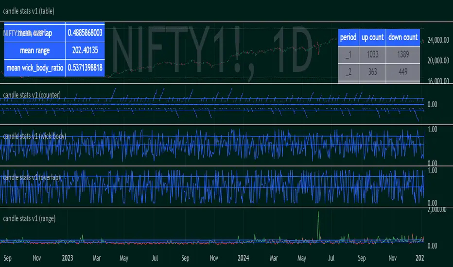
candle stats v1Objective:
Capture sequential/subsequent candle's relative properties
Average observations to represent the landscape of the marketplace
Parameters:
"range" : high-low
"overlap" : range - range
"wick_body_ratio" : (range - abs(open-close))/range
"up_count" for "period" : number of occurrences where consecutive candles have low>low . (note: the values are not cumulative over period)
*"down_count" for "period" : number of occurrences where consecutive candles have high<high . (note: the values are not cumulative over period)
** the last counter includes the value for "period" and all above
Basic inferences:
mean_range could be used to derive at an appropriate hard-stoploss
high wick to body ratio indicates healthy buzzing market, ie, each candle has a high frequency standing wave within it. a lower value indicates that the timeframe is ordered and highly directional
low overlap indicates trend definition/resolution
the counters show how likely or unlikely a run up or run down of a particular length is
a combination of counter and mean_range could be used to derive at an appropriate take profit
Use case:
to determine the appropriate timeframe to develop or apply a strategy
Future enhancements:
more complex relationships such as higher highs and lower lows
frequency of oscillations
DCStatCalcs_v0.1DCStatCalcs_v0.1 - Session-Based Statistical Projections
This Pine Script indicator overlays customizable horizontal lines on your chart to visualize a session's opening price and its statistical projections based on historical standard deviation (SD). Designed for traders who want to analyze price behavior within defined time sessions, it calculates and plots the session open price along with optional projection lines at 0.5, 1.0, 1.5, 2.0, and 2.5 standard deviations above and below the open, derived from past session data.
Key Features:
Customizable Sessions: Define your session time (e.g., 0600-1500) and timezone (e.g., America/New_York).
Historical Analysis: Uses a user-specified number of past sessions (default: 20) to compute the standard deviation of price movements relative to the session open.
Projection Lines: Displays toggleable lines at multiple SD levels with adjustable styles, colors, and widths for easy visualization.
Flexible Display: Extend lines beyond the current bar with an offset setting, and adjust label sizes for clarity.
Real-Time Updates: Lines dynamically extend as the session progresses, keeping projections relevant to the current bar.
How It Works:
At the start of each user-defined session, the indicator records the opening price and calculates the SD based on price deviations from the open across historical sessions. It then plots the open price line and, if enabled, projection lines at the specified SD intervals. These lines help traders identify potential support, resistance, or volatility zones based on statistical norms.
Use Case:
Ideal for day traders or analysts working with intraday charts to gauge price ranges and volatility within specific trading sessions, such as market opens or key economic hours.
Published under the Mozilla Public License 2.0. Created by dc_77.

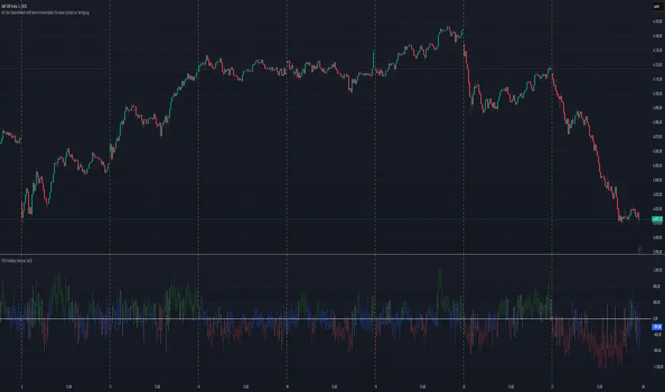
TICK Indikator
English:
The TICK Indicator measures in real time the number of up ticking stocks minus the number of down ticking stocks on the New York Stock Exchange (NYSE). It can display either the current TICK value ("Normal" mode) or the cumulative TICK values over the trading day ("Cumulative" mode). Positive values indicate market strength, while negative values signal weakness. Colored bars visualize momentum: green shades for rising, red for falling values. The zero line acts as a reference between buying and selling pressure.
Interpretation:
> +1000 and/or continuos lows above 0 → strong buying pressure
< -1000 and/or continuos highs below 0 → strong selling pressure
Around 0 → balanced market
Deutsch:
Der TICK Indikator misst in Echtzeit die Anzahl der Aktien, die an der New York Stock Exchange (NYSE) steigen, minus der Anzahl der fallenden Aktien. Der Indikator kann im "Normal"-Modus den aktuellen TICK-Wert anzeigen oder im "Cumulative"-Modus die kumulierten TICK-Werte über den Tag hinweg summieren. Positive Werte deuten auf eine allgemeine Markstärke hin, während negative Werte Schwäche signalisieren. Farbige Balken visualisieren die Dynamik: grüne Töne bei steigenden, rote bei fallenden Werten. Die Nullinie dient als Referenzpunkt zwischen Kauf- und Verkaufsdruck.
Interpretation:
> +1000 und/oder mehrere aufeinander folgende Tiefs über 0 → starker Kaufdruck
< -1000 und/oder mehrere aufeinander folgende Hochs unter 0 → starker Verkaufsdruck
Nahe 0 → ausgeglichener Markt
ValueAtTime█ OVERVIEW
This library is a Pine Script® programming tool for accessing historical values in a time series using UNIX timestamps . Its data structure and functions index values by time, allowing scripts to retrieve past values based on absolute timestamps or relative time offsets instead of relying on bar index offsets.
█ CONCEPTS
UNIX timestamps
In Pine Script®, a UNIX timestamp is an integer representing the number of milliseconds elapsed since January 1, 1970, at 00:00:00 UTC (the UNIX Epoch ). The timestamp is a unique, absolute representation of a specific point in time. Unlike a calendar date and time, a UNIX timestamp's meaning does not change relative to any time zone .
This library's functions process series values and corresponding UNIX timestamps in pairs , offering a simplified way to identify values that occur at or near distinct points in time instead of on specific bars.
Storing and retrieving time-value pairs
This library's `Data` type defines the structure for collecting time and value information in pairs. Objects of the `Data` type contain the following two fields:
• `times` – An array of "int" UNIX timestamps for each recorded value.
• `values` – An array of "float" values for each saved timestamp.
Each index in both arrays refers to a specific time-value pair. For instance, the `times` and `values` elements at index 0 represent the first saved timestamp and corresponding value. The library functions that maintain `Data` objects queue up to one time-value pair per bar into the object's arrays, where the saved timestamp represents the bar's opening time .
Because the `times` array contains a distinct UNIX timestamp for each item in the `values` array, it serves as a custom mapping for retrieving saved values. All the library functions that return information from a `Data` object use this simple two-step process to identify a value based on time:
1. Perform a binary search on the `times` array to find the earliest saved timestamp closest to the specified time or offset and get the element's index.
2. Access the element from the `values` array at the retrieved index, returning the stored value corresponding to the found timestamp.
Value search methods
There are several techniques programmers can use to identify historical values from corresponding timestamps. This library's functions include three different search methods to locate and retrieve values based on absolute times or relative time offsets:
Timestamp search
Find the value with the earliest saved timestamp closest to a specified timestamp.
Millisecond offset search
Find the value with the earliest saved timestamp closest to a specified number of milliseconds behind the current bar's opening time. This search method provides a time-based alternative to retrieving historical values at specific bar offsets.
Period offset search
Locate the value with the earliest saved timestamp closest to a defined period offset behind the current bar's opening time. The function calculates the span of the offset based on a period string . The "string" must contain one of the following unit tokens:
• "D" for days
• "W" for weeks
• "M" for months
• "Y" for years
• "YTD" for year-to-date, meaning the time elapsed since the beginning of the bar's opening year in the exchange time zone.
The period string can include a multiplier prefix for all supported units except "YTD" (e.g., "2W" for two weeks).
Note that the precise span covered by the "M", "Y", and "YTD" units varies across time. The "1M" period can cover 28, 29, 30, or 31 days, depending on the bar's opening month and year in the exchange time zone. The "1Y" period covers 365 or 366 days, depending on leap years. The "YTD" period's span changes with each new bar, because it always measures the time from the start of the current bar's opening year.
█ CALCULATIONS AND USE
This library's functions offer a flexible, structured approach to retrieving historical values at or near specific timestamps, millisecond offsets, or period offsets for different analytical needs.
See below for explanations of the exported functions and how to use them.
Retrieving single values
The library includes three functions that retrieve a single stored value using timestamp, millisecond offset, or period offset search methods:
• `valueAtTime()` – Locates the saved value with the earliest timestamp closest to a specified timestamp.
• `valueAtTimeOffset()` – Finds the saved value with the earliest timestamp closest to the specified number of milliseconds behind the current bar's opening time.
• `valueAtPeriodOffset()` – Finds the saved value with the earliest timestamp closest to the period-based offset behind the current bar's opening time.
Each function has two overloads for advanced and simple use cases. The first overload searches for a value in a user-specified `Data` object created by the `collectData()` function (see below). It returns a tuple containing the found value and the corresponding timestamp.
The second overload maintains a `Data` object internally to store and retrieve values for a specified `source` series. This overload returns a tuple containing the historical `source` value, the corresponding timestamp, and the current bar's `source` value, making it helpful for comparing past and present values from requested contexts.
Retrieving multiple values
The library includes the following functions to retrieve values from multiple historical points in time, facilitating calculations and comparisons with values retrieved across several intervals:
• `getDataAtTimes()` – Locates a past `source` value for each item in a `timestamps` array. Each retrieved value's timestamp represents the earliest time closest to one of the specified timestamps.
• `getDataAtTimeOffsets()` – Finds a past `source` value for each item in a `timeOffsets` array. Each retrieved value's timestamp represents the earliest time closest to one of the specified millisecond offsets behind the current bar's opening time.
• `getDataAtPeriodOffsets()` – Finds a past value for each item in a `periods` array. Each retrieved value's timestamp represents the earliest time closest to one of the specified period offsets behind the current bar's opening time.
Each function returns a tuple with arrays containing the found `source` values and their corresponding timestamps. In addition, the tuple includes the current `source` value and the symbol's description, which also makes these functions helpful for multi-interval comparisons using data from requested contexts.
Processing period inputs
When writing scripts that retrieve historical values based on several user-specified period offsets, the most concise approach is to create a single text input that allows users to list each period, then process the "string" list into an array for use in the `getDataAtPeriodOffsets()` function.
This library includes a `getArrayFromString()` function to provide a simple way to process strings containing comma-separated lists of periods. The function splits the specified `str` by its commas and returns an array containing every non-empty item in the list with surrounding whitespaces removed. View the example code to see how we use this function to process the value of a text area input .
Calculating period offset times
Because the exact amount of time covered by a specified period offset can vary, it is often helpful to verify the resulting times when using the `valueAtPeriodOffset()` or `getDataAtPeriodOffsets()` functions to ensure the calculations work as intended for your use case.
The library's `periodToTimestamp()` function calculates an offset timestamp from a given period and reference time. With this function, programmers can verify the time offsets in a period-based data search and use the calculated offset times in additional operations.
For periods with "D" or "W" units, the function calculates the time offset based on the absolute number of milliseconds the period covers (e.g., `86400000` for "1D"). For periods with "M", "Y", or "YTD" units, the function calculates an offset time based on the reference time's calendar date in the exchange time zone.
Collecting data
All the `getDataAt*()` functions, and the second overloads of the `valueAt*()` functions, collect and maintain data internally, meaning scripts do not require a separate `Data` object when using them. However, the first overloads of the `valueAt*()` functions do not collect data, because they retrieve values from a user-specified `Data` object.
For cases where a script requires a separate `Data` object for use with these overloads or other custom routines, this library exports the `collectData()` function. This function queues each bar's `source` value and opening timestamp into a `Data` object and returns the object's ID.
This function is particularly useful when searching for values from a specific series more than once. For instance, instead of using multiple calls to the second overloads of `valueAt*()` functions with the same `source` argument, programmers can call `collectData()` to store each bar's `source` and opening timestamp, then use the returned `Data` object's ID in calls to the first `valueAt*()` overloads to reduce memory usage.
The `collectData()` function and all the functions that collect data internally include two optional parameters for limiting the saved time-value pairs to a sliding window: `timeOffsetLimit` and `timeframeLimit`. When either has a non-na argument, the function restricts the collected data to the maximum number of recent bars covered by the specified millisecond- and timeframe-based intervals.
NOTE : All calls to the functions that collect data for a `source` series can execute up to once per bar or realtime tick, because each stored value requires a unique corresponding timestamp. Therefore, scripts cannot call these functions iteratively within a loop . If a call to these functions executes more than once inside a loop's scope, it causes a runtime error.
█ EXAMPLE CODE
The example code at the end of the script demonstrates one possible use case for this library's functions. The code retrieves historical price data at user-specified period offsets, calculates price returns for each period from the retrieved data, and then populates a table with the results.
The example code's process is as follows:
1. Input a list of periods – The user specifies a comma-separated list of period strings in the script's "Period list" input (e.g., "1W, 1M, 3M, 1Y, YTD"). Each item in the input list represents a period offset from the latest bar's opening time.
2. Process the period list – The example calls `getArrayFromString()` on the first bar to split the input list by its commas and construct an array of period strings.
3. Request historical data – The code uses a call to `getDataAtPeriodOffsets()` as the `expression` argument in a request.security() call to retrieve the closing prices of "1D" bars for each period included in the processed `periods` array.
4. Display information in a table – On the latest bar, the code uses the retrieved data to calculate price returns over each specified period, then populates a two-row table with the results. The cells for each return percentage are color-coded based on the magnitude and direction of the price change. The cells also include tooltips showing the compared daily bar's opening date in the exchange time zone.
█ NOTES
• This library's architecture relies on a user-defined type (UDT) for its data storage format. UDTs are blueprints from which scripts create objects , i.e., composite structures with fields containing independent values or references of any supported type.
• The library functions search through a `Data` object's `times` array using the array.binary_search_leftmost() function, which is more efficient than looping through collected data to identify matching timestamps. Note that this built-in works only for arrays with elements sorted in ascending order .
• Each function that collects data from a `source` series updates the values and times stored in a local `Data` object's arrays. If a single call to these functions were to execute in a loop , it would store multiple values with an identical timestamp, which can cause erroneous search behavior. To prevent looped calls to these functions, the library uses the `checkCall()` helper function in their scopes. This function maintains a counter that increases by one each time it executes on a confirmed bar. If the count exceeds the total number of bars, indicating the call executes more than once in a loop, it raises a runtime error .
• Typically, when requesting higher-timeframe data with request.security() while using barmerge.lookahead_on as the `lookahead` argument, the `expression` argument should be offset with the history-referencing operator to prevent lookahead bias on historical bars. However, the call in this script's example code enables lookahead without offsetting the `expression` because the script displays results only on the last historical bar and all realtime bars, where there is no future data to leak into the past. This call ensures the displayed results use the latest data available from the context on realtime bars.
Look first. Then leap.
█ EXPORTED TYPES
Data
A structure for storing successive timestamps and corresponding values from a dataset.
Fields:
times (array) : An "int" array containing a UNIX timestamp for each value in the `values` array.
values (array) : A "float" array containing values corresponding to the timestamps in the `times` array.
█ EXPORTED FUNCTIONS
getArrayFromString(str)
Splits a "string" into an array of substrings using the comma (`,`) as the delimiter. The function trims surrounding whitespace characters from each substring, and it excludes empty substrings from the result.
Parameters:
str (series string) : The "string" to split into an array based on its commas.
Returns: (array) An array of trimmed substrings from the specified `str`.
periodToTimestamp(period, referenceTime)
Calculates a UNIX timestamp representing the point offset behind a reference time by the amount of time within the specified `period`.
Parameters:
period (series string) : The period string, which determines the time offset of the returned timestamp. The specified argument must contain a unit and an optional multiplier (e.g., "1Y", "3M", "2W", "YTD"). Supported units are:
- "Y" for years.
- "M" for months.
- "W" for weeks.
- "D" for days.
- "YTD" (Year-to-date) for the span from the start of the `referenceTime` value's year in the exchange time zone. An argument with this unit cannot contain a multiplier.
referenceTime (series int) : The millisecond UNIX timestamp from which to calculate the offset time.
Returns: (int) A millisecond UNIX timestamp representing the offset time point behind the `referenceTime`.
collectData(source, timeOffsetLimit, timeframeLimit)
Collects `source` and `time` data successively across bars. The function stores the information within a `Data` object for use in other exported functions/methods, such as `valueAtTimeOffset()` and `valueAtPeriodOffset()`. Any call to this function cannot execute more than once per bar or realtime tick.
Parameters:
source (series float) : The source series to collect. The function stores each value in the series with an associated timestamp representing its corresponding bar's opening time.
timeOffsetLimit (simple int) : Optional. A time offset (range) in milliseconds. If specified, the function limits the collected data to the maximum number of bars covered by the range, with a minimum of one bar. If the call includes a non-empty `timeframeLimit` value, the function limits the data using the largest number of bars covered by the two ranges. The default is `na`.
timeframeLimit (simple string) : Optional. A valid timeframe string. If specified and not empty, the function limits the collected data to the maximum number of bars covered by the timeframe, with a minimum of one bar. If the call includes a non-na `timeOffsetLimit` value, the function limits the data using the largest number of bars covered by the two ranges. The default is `na`.
Returns: (Data) A `Data` object containing collected `source` values and corresponding timestamps over the allowed time range.
method valueAtTime(data, timestamp)
(Overload 1 of 2) Retrieves value and time data from a `Data` object's fields at the index of the earliest timestamp closest to the specified `timestamp`. Callable as a method or a function.
Parameters:
data (series Data) : The `Data` object containing the collected time and value data.
timestamp (series int) : The millisecond UNIX timestamp to search. The function returns data for the earliest saved timestamp that is closest to the value.
Returns: ( ) A tuple containing the following data from the `Data` object:
- The stored value corresponding to the identified timestamp ("float").
- The earliest saved timestamp that is closest to the specified `timestamp` ("int").
valueAtTime(source, timestamp, timeOffsetLimit, timeframeLimit)
(Overload 2 of 2) Retrieves `source` and time information for the earliest bar whose opening timestamp is closest to the specified `timestamp`. Any call to this function cannot execute more than once per bar or realtime tick.
Parameters:
source (series float) : The source series to analyze. The function stores each value in the series with an associated timestamp representing its corresponding bar's opening time.
timestamp (series int) : The millisecond UNIX timestamp to search. The function returns data for the earliest bar whose timestamp is closest to the value.
timeOffsetLimit (simple int) : Optional. A time offset (range) in milliseconds. If specified, the function limits the collected data to the maximum number of bars covered by the range, with a minimum of one bar. If the call includes a non-empty `timeframeLimit` value, the function limits the data using the largest number of bars covered by the two ranges. The default is `na`.
timeframeLimit (simple string) : (simple string) Optional. A valid timeframe string. If specified and not empty, the function limits the collected data to the maximum number of bars covered by the timeframe, with a minimum of one bar. If the call includes a non-na `timeOffsetLimit` value, the function limits the data using the largest number of bars covered by the two ranges. The default is `na`.
Returns: ( ) A tuple containing the following data:
- The `source` value corresponding to the identified timestamp ("float").
- The earliest bar's timestamp that is closest to the specified `timestamp` ("int").
- The current bar's `source` value ("float").
method valueAtTimeOffset(data, timeOffset)
(Overload 1 of 2) Retrieves value and time data from a `Data` object's fields at the index of the earliest saved timestamp closest to `timeOffset` milliseconds behind the current bar's opening time. Callable as a method or a function.
Parameters:
data (series Data) : The `Data` object containing the collected time and value data.
timeOffset (series int) : The millisecond offset behind the bar's opening time. The function returns data for the earliest saved timestamp that is closest to the calculated offset time.
Returns: ( ) A tuple containing the following data from the `Data` object:
- The stored value corresponding to the identified timestamp ("float").
- The earliest saved timestamp that is closest to `timeOffset` milliseconds before the current bar's opening time ("int").
valueAtTimeOffset(source, timeOffset, timeOffsetLimit, timeframeLimit)
(Overload 2 of 2) Retrieves `source` and time information for the earliest bar whose opening timestamp is closest to `timeOffset` milliseconds behind the current bar's opening time. Any call to this function cannot execute more than once per bar or realtime tick.
Parameters:
source (series float) : The source series to analyze. The function stores each value in the series with an associated timestamp representing its corresponding bar's opening time.
timeOffset (series int) : The millisecond offset behind the bar's opening time. The function returns data for the earliest bar's timestamp that is closest to the calculated offset time.
timeOffsetLimit (simple int) : Optional. A time offset (range) in milliseconds. If specified, the function limits the collected data to the maximum number of bars covered by the range, with a minimum of one bar. If the call includes a non-empty `timeframeLimit` value, the function limits the data using the largest number of bars covered by the two ranges. The default is `na`.
timeframeLimit (simple string) : Optional. A valid timeframe string. If specified and not empty, the function limits the collected data to the maximum number of bars covered by the timeframe, with a minimum of one bar. If the call includes a non-na `timeOffsetLimit` value, the function limits the data using the largest number of bars covered by the two ranges. The default is `na`.
Returns: ( ) A tuple containing the following data:
- The `source` value corresponding to the identified timestamp ("float").
- The earliest bar's timestamp that is closest to `timeOffset` milliseconds before the current bar's opening time ("int").
- The current bar's `source` value ("float").
method valueAtPeriodOffset(data, period)
(Overload 1 of 2) Retrieves value and time data from a `Data` object's fields at the index of the earliest timestamp closest to a calculated offset behind the current bar's opening time. The calculated offset represents the amount of time covered by the specified `period`. Callable as a method or a function.
Parameters:
data (series Data) : The `Data` object containing the collected time and value data.
period (series string) : The period string, which determines the calculated time offset. The specified argument must contain a unit and an optional multiplier (e.g., "1Y", "3M", "2W", "YTD"). Supported units are:
- "Y" for years.
- "M" for months.
- "W" for weeks.
- "D" for days.
- "YTD" (Year-to-date) for the span from the start of the current bar's year in the exchange time zone. An argument with this unit cannot contain a multiplier.
Returns: ( ) A tuple containing the following data from the `Data` object:
- The stored value corresponding to the identified timestamp ("float").
- The earliest saved timestamp that is closest to the calculated offset behind the bar's opening time ("int").
valueAtPeriodOffset(source, period, timeOffsetLimit, timeframeLimit)
(Overload 2 of 2) Retrieves `source` and time information for the earliest bar whose opening timestamp is closest to a calculated offset behind the current bar's opening time. The calculated offset represents the amount of time covered by the specified `period`. Any call to this function cannot execute more than once per bar or realtime tick.
Parameters:
source (series float) : The source series to analyze. The function stores each value in the series with an associated timestamp representing its corresponding bar's opening time.
period (series string) : The period string, which determines the calculated time offset. The specified argument must contain a unit and an optional multiplier (e.g., "1Y", "3M", "2W", "YTD"). Supported units are:
- "Y" for years.
- "M" for months.
- "W" for weeks.
- "D" for days.
- "YTD" (Year-to-date) for the span from the start of the current bar's year in the exchange time zone. An argument with this unit cannot contain a multiplier.
timeOffsetLimit (simple int) : Optional. A time offset (range) in milliseconds. If specified, the function limits the collected data to the maximum number of bars covered by the range, with a minimum of one bar. If the call includes a non-empty `timeframeLimit` value, the function limits the data using the largest number of bars covered by the two ranges. The default is `na`.
timeframeLimit (simple string) : Optional. A valid timeframe string. If specified and not empty, the function limits the collected data to the maximum number of bars covered by the timeframe, with a minimum of one bar. If the call includes a non-na `timeOffsetLimit` value, the function limits the data using the largest number of bars covered by the two ranges. The default is `na`.
Returns: ( ) A tuple containing the following data:
- The `source` value corresponding to the identified timestamp ("float").
- The earliest bar's timestamp that is closest to the calculated offset behind the current bar's opening time ("int").
- The current bar's `source` value ("float").
getDataAtTimes(timestamps, source, timeOffsetLimit, timeframeLimit)
Retrieves `source` and time information for each bar whose opening timestamp is the earliest one closest to one of the UNIX timestamps specified in the `timestamps` array. Any call to this function cannot execute more than once per bar or realtime tick.
Parameters:
timestamps (array) : An array of "int" values representing UNIX timestamps. The function retrieves `source` and time data for each element in this array.
source (series float) : The source series to analyze. The function stores each value in the series with an associated timestamp representing its corresponding bar's opening time.
timeOffsetLimit (simple int) : Optional. A time offset (range) in milliseconds. If specified, the function limits the collected data to the maximum number of bars covered by the range, with a minimum of one bar. If the call includes a non-empty `timeframeLimit` value, the function limits the data using the largest number of bars covered by the two ranges. The default is `na`.
timeframeLimit (simple string) : Optional. A valid timeframe string. If specified and not empty, the function limits the collected data to the maximum number of bars covered by the timeframe, with a minimum of one bar. If the call includes a non-na `timeOffsetLimit` value, the function limits the data using the largest number of bars covered by the two ranges. The default is `na`.
Returns: ( ) A tuple of the following data:
- An array containing a `source` value for each identified timestamp (array).
- An array containing an identified timestamp for each item in the `timestamps` array (array).
- The current bar's `source` value ("float").
- The symbol's description from `syminfo.description` ("string").
getDataAtTimeOffsets(timeOffsets, source, timeOffsetLimit, timeframeLimit)
Retrieves `source` and time information for each bar whose opening timestamp is the earliest one closest to one of the time offsets specified in the `timeOffsets` array. Each offset in the array represents the absolute number of milliseconds behind the current bar's opening time. Any call to this function cannot execute more than once per bar or realtime tick.
Parameters:
timeOffsets (array) : An array of "int" values representing the millisecond time offsets used in the search. The function retrieves `source` and time data for each element in this array. For example, the array ` ` specifies that the function returns data for the timestamps closest to one day and one week behind the current bar's opening time.
source (float) : (series float) The source series to analyze. The function stores each value in the series with an associated timestamp representing its corresponding bar's opening time.
timeOffsetLimit (simple int) : Optional. A time offset (range) in milliseconds. If specified, the function limits the collected data to the maximum number of bars covered by the range, with a minimum of one bar. If the call includes a non-empty `timeframeLimit` value, the function limits the data using the largest number of bars covered by the two ranges. The default is `na`.
timeframeLimit (simple string) : Optional. A valid timeframe string. If specified and not empty, the function limits the collected data to the maximum number of bars covered by the timeframe, with a minimum of one bar. If the call includes a non-na `timeOffsetLimit` value, the function limits the data using the largest number of bars covered by the two ranges. The default is `na`.
Returns: ( ) A tuple of the following data:
- An array containing a `source` value for each identified timestamp (array).
- An array containing an identified timestamp for each offset specified in the `timeOffsets` array (array).
- The current bar's `source` value ("float").
- The symbol's description from `syminfo.description` ("string").
getDataAtPeriodOffsets(periods, source, timeOffsetLimit, timeframeLimit)
Retrieves `source` and time information for each bar whose opening timestamp is the earliest one closest to a calculated offset behind the current bar's opening time. Each calculated offset represents the amount of time covered by a period specified in the `periods` array. Any call to this function cannot execute more than once per bar or realtime tick.
Parameters:
periods (array) : An array of period strings, which determines the time offsets used in the search. The function retrieves `source` and time data for each element in this array. For example, the array ` ` specifies that the function returns data for the timestamps closest to one day, week, and month behind the current bar's opening time. Each "string" in the array must contain a unit and an optional multiplier. Supported units are:
- "Y" for years.
- "M" for months.
- "W" for weeks.
- "D" for days.
- "YTD" (Year-to-date) for the span from the start of the current bar's year in the exchange time zone. An argument with this unit cannot contain a multiplier.
source (float) : (series float) The source series to analyze. The function stores each value in the series with an associated timestamp representing its corresponding bar's opening time.
timeOffsetLimit (simple int) : Optional. A time offset (range) in milliseconds. If specified, the function limits the collected data to the maximum number of bars covered by the range, with a minimum of one bar. If the call includes a non-empty `timeframeLimit` value, the function limits the data using the largest number of bars covered by the two ranges. The default is `na`.
timeframeLimit (simple string) : Optional. A valid timeframe string. If specified and not empty, the function limits the collected data to the maximum number of bars covered by the timeframe, with a minimum of one bar. If the call includes a non-na `timeOffsetLimit` value, the function limits the data using the largest number of bars covered by the two ranges. The default is `na`.
Returns: ( ) A tuple of the following data:
- An array containing a `source` value for each identified timestamp (array).
- An array containing an identified timestamp for each period specified in the `periods` array (array).
- The current bar's `source` value ("float").
- The symbol's description from `syminfo.description` ("string").

Price Change IndicatorPrice Change Indicator (PCI)
Version: 1.0
Author: LazyTrader 🚀
🔍 Overview
The Price Change Indicator (PCI) helps traders visualize and compare price changes between the current bar and the previous bar. It provides a customizable display of price changes in two formats:
Percentage (%) Change – Relative price movement.
Natural Change – Absolute difference in price units.
⚙️ Key Features
✅ Customizable Calculation Method: Choose how the price change is calculated:
Opening Price
Closing Price
High
Low
✅ Flexible Display Format:
Show Percentage (%) Change.
Show Natural (Absolute) Change in price.
✅ Adjustable Sensitivity with Multiplier:
100 (Standard Change)
1000 (Small Change)
10000 (Tiny Change)
✅ Intuitive Labeling:
Green label (above bar) for increase.
Red label (below bar) for decrease.
No label if no change.
Large, easy-to-read labels for better visibility.
✅ Perfect for Any Market:
Stocks 📈
Forex 💱
Crypto 🚀
Commodities 🛢️
📊 How It Works
The indicator calculates the difference between the current and previous bar’s price based on your chosen method.
The result is displayed as either a percentage (%) or a natural price change.
If the price has increased, a green label is displayed above the bar.
If the price has decreased, a red label is displayed below the bar.
⚡ How to Use
Add the indicator to your chart.
Go to settings and customize:
Select calculation method (Open, Close, High, Low).
Choose display format (% or Natural Change).
Adjust multiplier for more sensitivity.
Analyze the labels to see price movements easily!
🔧 Settings Explained
Setting Description
Price Calculation Method: Choose Open, Close, High, or Low price for comparison.
Display Format: Show either % Change or Natural Change.
Multiplier: Apply 100, 1000, or 10000 to scale small price changes.
Show Labels: Toggle labels on/off.
🎯 Best Use Cases
🔹 Identifying strong price movements
🔹 Spotting trends and momentum shifts
🔹 Comparing price movement intensity
🔹 Works for scalping, swing trading, and long-term analysis

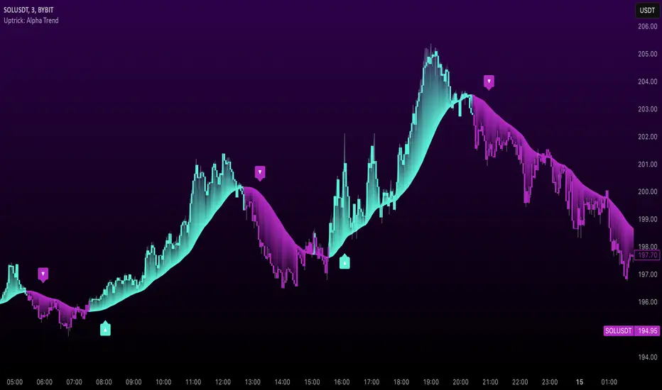
Uptrick: Alpha TrendIntroduction
Uptrick: Alpha Trend is a comprehensive technical analysis indicator designed to provide traders with detailed insights into market trends, momentum, and risk metrics. It adapts to various trading styles—from quick scalps to longer-term positions—by dynamically adjusting its calculations and visual elements. By combining multiple smoothing techniques, advanced color schemes, and customizable data tables, the indicator offers a holistic view of market behavior.
Originality
The Alpha Trend indicator distinguishes itself by blending established technical concepts with innovative adaptations. It employs three different smoothing techniques tailored to specific trading modes (Scalp, Swing, and Position), and it dynamically adjusts its parameters to match the chosen mode. The indicator also offers a wide range of color palettes and multiple on-screen tables that display key metrics. This unique combination of features, along with its ability to adapt in real time, sets it apart as a versatile tool for both novice and experienced traders.
Features
1. Multi-Mode Trend Line
The indicator automatically selects a smoothing method based on the trading mode:
- Scalp Mode uses the Hull Moving Average (HMA) for rapid responsiveness.
- Swing Mode employs the Exponential Moving Average (EMA) for balanced reactivity.
- Position Mode applies the Weighted Moving Average (WMA) for smoother, long-term trends.
Each method is chosen to best capture the price action dynamics appropriate to the trader’s timeframe.
2. Adaptive Momentum Thresholds
It tracks bullish and bearish momentum with counters that increment as the trend confirms directional movement. When these counters exceed a user-defined threshold, the indicator generates optional buy or sell signals. This approach helps filter out minor fluctuations and highlights significant market moves.
3. Gradient Fills
Two types of fills enhance visual clarity:
- Standard Gradient Fill displays ATR-based zones above and below the trend line, indicating potential bullish and bearish areas.
- Fading Gradient Fill creates a smooth transition between the trend line and the price, visually emphasizing the distance between them.
4. Bar Coloring and Signal Markers
The indicator can color-code bars based on market conditions—bullish, bearish, or neutral—allowing for immediate visual assessment. Additionally, signal markers such as buy and sell arrows are plotted when momentum thresholds are breached.
5. Comprehensive Data Tables
Uptrick: Alpha Trend offers several optional tables for detailed analysis:
- Insider Info: Displays key metrics like the current trend value, bullish/bearish momentum counts, and ATR.
- Indicator Metrics: Lists input settings such as trend length, damping, signal threshold, and net momentum.
- Market Analysis: Summarizes overall trend direction, trend strength, Sortino ratio, return, and volatility.
- Price & Trend Dynamics: Details price deviation from the trend, trend slope, and ATR ratio.
- Momentum & Volatility Insights: Presents RSI, standard deviation (volatility), and net momentum.
- Performance & Acceleration Metrics: Focuses on the Sortino ratio, trend acceleration, return, and trend strength.
Each table can be positioned flexibly on the chart, allowing traders to customize the layout according to their needs.
Why It Combines Specific Smoothing Techniques
Smoothing techniques are essential for filtering out market noise and revealing underlying trends. The indicator combines three smoothing methods for the following reasons:
- The Hull Moving Average (HMA) in Scalp Mode minimizes lag and responds quickly to price changes, which is critical for short-term trading.
- The Exponential Moving Average (EMA) in Swing Mode gives more weight to recent data, striking a balance between speed and smoothness. This makes it suitable for mid-term trend analysis.
- The Weighted Moving Average (WMA) in Position Mode smooths out short-term fluctuations, offering a clear view of longer-term trends and reducing the impact of transient market volatility.
By using these specific methods in their respective trading modes, the indicator ensures that the trend line is appropriately responsive for the intended time frame, enhancing decision-making while maintaining clarity.
Inputs
1. Trend Length (Default: 30)
Defines the lookback period for the smoothing calculation. A shorter trend length results in a more responsive line, while a longer length produces a smoother, less volatile trend.
2. Trend Damping (Default: 0.75)
Controls the degree of smoothing applied to the trend line. Lower values lead to a smoother curve, whereas higher values increase sensitivity to price fluctuations.
3. Signal Strength Threshold (Default: 5)
Specifies the number of consecutive bullish or bearish bars required to trigger a signal. Higher thresholds reduce the frequency of signals, focusing on stronger moves.
4. Enable Bar Coloring (Default: True)
Toggles whether each price bar is colored to indicate bullish, bearish, or neutral conditions.
5. Enable Signals (Default: True)
When enabled, this option plots buy or sell arrows on the chart once the momentum thresholds are met.
6. Enable Standard Gradient Fill (Default: False)
Activates ATR-based gradient fills around the trend line to visualize potential support and resistance zones.
7. Enable Fading Gradient Fill (Default: True)
Draws a gradual color transition between the trend line and the current price, emphasizing their divergence.
8. Trading Mode (Options: Scalp, Swing, Position)
Determines which smoothing method and ATR period to use, adapting the indicator’s behavior to short-term, medium-term, or long-term trading.
9. Table Position Inputs
Allows users to select from nine possible chart positions (top, middle, bottom; left, center, right) for each data table.
10. Show Table Booleans
Separate toggles control the display of each table (Insider Info, Indicator Metrics, Market Analysis, and the three Deep Tables), enabling a customized view of the data.
Color Schemes
(Default) - The colors in the preview image of the indicator.
(Emerald)
(Sapphire)
(Golden Blaze)
(Mystic)
(Monochrome)
(Pastel)
(Vibrant)
(Earth)
(Neon)
Calculations
1. Trend Line Methods
- Scalp Mode: Utilizes the Hull Moving Average (HMA), which computes two weighted moving averages (one at half the length and one at full length), subtracts them, and then applies a final weighted average based on the square root of the length. This method minimizes lag and increases responsiveness.
- Swing Mode: Uses the Exponential Moving Average (EMA), which assigns greater weight to recent prices, thus balancing quick reaction with smoothness.
- Position Mode: Applies the Weighted Moving Average (WMA) to focus on longer-term trends by emphasizing the entire lookback period and reducing the impact of short-term volatility.
2. Momentum Tracking
The indicator maintains separate counters for bullish and bearish momentum. These counters increase as the trend confirms directional movement and reset when the trend reverses. When a counter exceeds the defined signal strength threshold, a corresponding signal (buy or sell) is triggered.
3. Volatility and ATR Zones
The Average True Range (ATR) is calculated using a period that adapts to the selected trading mode (shorter for Scalp, longer for Position). The ATR value is then used to define upper and lower zones around the trend line, highlighting the current level of market volatility.
4. Return and Trend Acceleration
- Return is calculated as the difference between the current and previous closing prices, providing a simple measure of price change.
- Trend Acceleration is derived from the change in the trend line’s movement (its first derivative) compared to the previous bar. This metric indicates whether the trend is gaining or losing momentum.
5. Sortino Ratio and Standard Deviation
- The Sortino Ratio measures risk-adjusted performance by comparing returns to downside volatility (only considering negative price changes).
- Standard Deviation is computed over the lookback period to assess the extent of price fluctuations, offering insights into market stability.
Usage
This indicator is suitable for various time frames and market instruments. Traders can enable or disable specific visual elements such as gradient fills, bar coloring, and signal markers based on their preference. For a minimalist approach, one might choose to display only the primary trend line. For a deeper analysis, enabling multiple tables can provide extensive data on momentum, volatility, trend dynamics, and risk metrics.
Important Note on Risk
Trading involves inherent risk, and no indicator can eliminate the uncertainty of the markets. Past performance is not indicative of future results. It is essential to use proper risk management, test any new tool thoroughly, and consult multiple sources or professional advice before making trading decisions.
Conclusion
Uptrick: Alpha Trend unifies a diverse set of calculations, adaptive smoothing techniques, and customizable visual elements into one powerful tool. By combining the Hull, Exponential, and Weighted Moving Averages, the indicator is able to provide a trend line that is both responsive and smooth, depending on the trading mode. Its advanced color schemes, gradient fills, and detailed data tables deliver a comprehensive analysis of market trends, momentum, and risk. Whether you are a short-term trader or a long-term investor, this indicator aims to clarify price action and assist you in making more informed trading decisions.
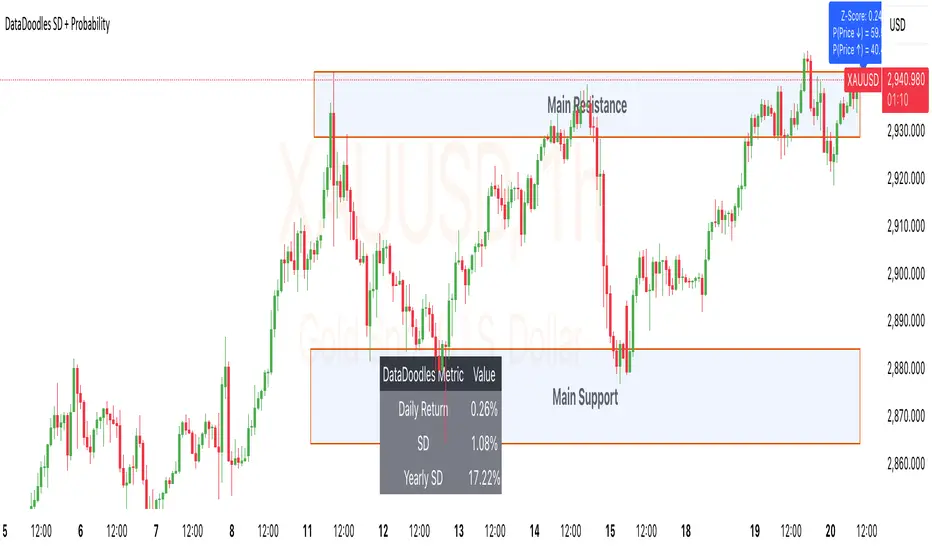
DataDoodles SD + ProbabilityDataDoodles SD + Probability
Overview:
The “DataDoodles SD + Probability” indicator is designed to provide traders with a statistical edge by leveraging standard deviation and probability metrics. This advanced tool calculates the annualized standard deviation, Z-score, and probability of price movements, offering insights into potential market direction with customizable alert thresholds.
Key Features:
1. Annualized Standard Deviation (Volatility) Calculation:
• Uses a user-defined period to compute the rolling standard deviation of daily returns.
• Annualizes the volatility, giving a clear picture of expected price fluctuations.
2. Probability of Price Movement:
• Calculates the probability of price moving up or down using a corrected Z-Score.
• Displays the probability percentage for both upward and downward movements.
3. Dynamic Alerts:
• Configurable alerts for upward and downward price movement probabilities.
• Receive alerts when the probability exceeds user-defined thresholds.
4. Projections and Visuals:
• Plots projected high and low price levels based on annualized volatility.
• Displays Z-Score and probability metrics on the chart for quick reference.
5. Comprehensive Data Table:
• Bottom-center table displays key metrics:
• Daily Return
• Standard Deviation (SD)
• Annualized Standard Deviation (Yearly SD)
User Inputs:
• Annualization Period: Set the time frame for volatility annualization (Default: 252 days).
• SD Period: Define the rolling window for calculating standard deviation (Default: 252 days).
• Alert Probability Up/Down: Customize the probability thresholds for alerts (Default: 90%).
How It Works:
• Data Request and Calculation:
• Uses daily close prices to ensure consistent timeframe calculations.
• Calculates daily returns and annualizes the volatility using the square root of the time frame.
• Probability Computation:
• Employs a normal distribution CDF approximation to compute the probability of upward and downward price movements.
• Adjusts probabilities based on Z-Score to ensure accuracy.
• High and Low Projections:
• Utilizes the annualized volatility to estimate high and low price projections for the year.
• Visual Indicators and Alerts:
• Plots projected high (green) and low (red) levels on the chart.
• Displays Z-Score, probability percentages, and dynamically updates a statistics table.
Use Cases:
• Trend Analysis: Identify high-probability market movements using the probability metrics.
• Volatility Insights: Understand annualized volatility to gauge market risk and potential price ranges.
• Strategic Trading Decisions: Set alerts for high-probability scenarios to optimize entry and exit points.
Why Use “DataDoodles SD + Probability”?
This indicator provides a powerful combination of statistical analysis and visual representation. It empowers traders with:
• Quantitative Edge: By leveraging probability metrics and standard deviation, users can make informed trading decisions.
• Risk Management: Annualized volatility projections help in setting realistic stop-loss and take-profit levels.
• Actionable Alerts: Customizable probability alerts ensure users are notified of potential market moves, allowing proactive trading strategies.
Recommended Settings:
• Annualization Period: 252 (Ideal for daily data representing a trading year)
• SD Period: 252 (One trading year for consistent volatility calculations)
• Alert Probability: Set to 90% for conservative signals or lower for more frequent alerts.
Final Thoughts:
The “DataDoodles SD + Probability” indicator is a robust tool for traders looking to integrate statistical analysis into their trading strategies. It combines volatility measurement, probability calculations, and dynamic alerts to provide a comprehensive market overview.
Whether you’re a day trader or a long-term investor, this indicator can enhance your market insight and improve decision-making accuracy.
Disclaimer:
This indicator is a technical analysis tool designed for educational purposes. Past performance is not indicative of future results. Traders are encouraged to perform their own analysis and manage risk accordingly.
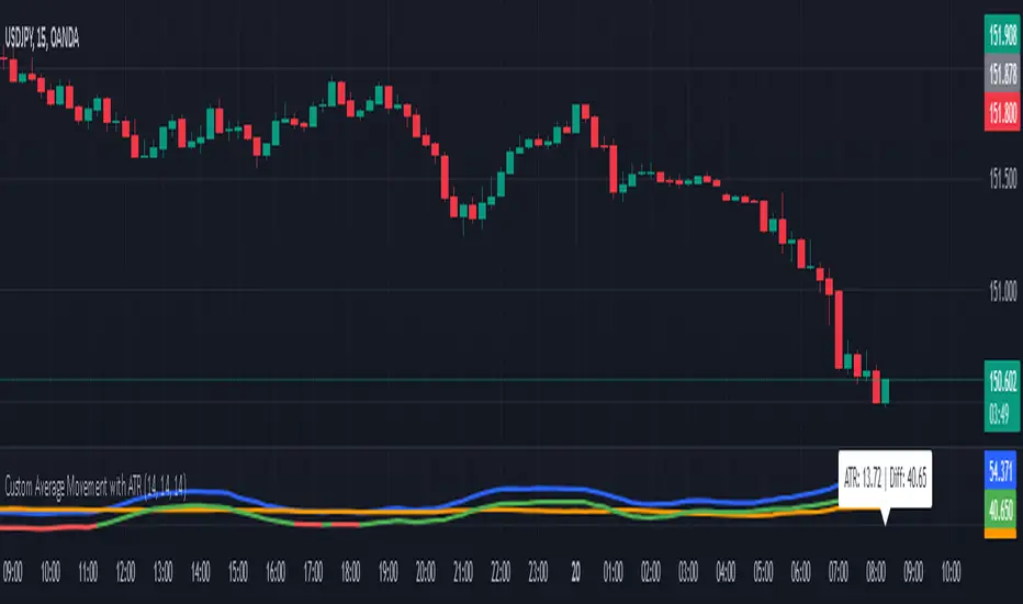
Average Pips MovementMarket average pips Movement and sideways detection
Why this indicator:
It detects sideways or no movements of the market
It helps to know the pips values being changed during the given ranges, so traders know how much pips market can go down or up and set their trade for suitable time frame.
Settings:
You can change the atr values and range values. both are indicating how many bars to consider for the average. I suggest to uncheck the lables and labels on price scale to keep the chart nice and fresh.
You can also change the colors for each line.
Use Cases:
First value, indicating ranges average, the pips value you can expect to go up or down during this time. lower time frame means lower number. This is the key point. It shows the risk you might jumped to. if you can risk and target only 20pips and this value is 50pips, go down few time frame and find the 20 value. so you will be safe.
Second value, is just normal atr for reference only.
Third value, is the difference of atr and range values, closer to zero or negative value means no movement in the market. it happens at the end of new york session till the open of tokyo sessions and sometimes extended till london sessions open. Higher the number, the more movements in the market.
This indicator is mainly for the begginers. If you already know the best time frame for you to trade and when the market moving, you do not need this indicator at all.
And also disclaimer: this indicator doesn't show the pips values you will make profit, the value are just for references and it is calculated based on the market movement, so you know the things only once it occured!
Thanks!
Btc and Eth 5 min winnerWhat the Strategy Does
Finding the Trend (Like Watching the Bus Move): The strategy uses special tools called Hull Moving Averages (HMAs) to figure out if Bitcoin (BTC) Ethereum (ETH) prices are generally going up or down. It looks at short-term (5 minutes) and long-term (10 minutes) price movements to make sure the “bus” (the market) is moving strongly in one direction—up for buying, down for selling.
Spotting Good Times to Jump On (Buy or Sell Signals): It looks for two types of opportunities:
Pullbacks: When the price dips a little while still moving up (like the bus slowing down but not stopping), it’s a chance to buy.
Breakouts: When the price suddenly jumps higher after being stuck (like the bus speeding up), it’s another chance to buy. It does the opposite for selling when prices are dropping.
It also checks if there’s enough “passenger activity” (volume) and momentum (speed of price change) to make sure it’s a good move.
Avoiding Traffic Jams (Filters): The strategy uses tools like RSI (to check if the market’s too fast or too slow), volume (to see if enough people are trading), and ATR (to measure how wild the price swings are). It skips trades if things look too chaotic or if the trend isn’t strong enough.
Setting Safety Stops and Profit Targets: Once you’re on the “bus,” it sets rules to protect you:
Stop-Loss: If the price moves against you by a small amount (0.5% of the typical price swing), you jump off to avoid losing too much—think of it as getting off before the bus crashes.
Take-Profit: If the price moves in your favor by a small amount (1.0% of the typical swing), you cash out—imagine getting off at your stop with a profit.
Trailing Stop: If the price keeps moving your way, it adjusts your exit point to lock in more profit, like moving your stop closer as the bus keeps going.
Using Leverage (10x Boost): This strategy uses 10x leverage on Binance futures, meaning for every $1 you have, you trade like you have $10. This can make profits (or losses) 10 times bigger, so it’s risky but can be rewarding if you’re careful.
Why 5 Minutes and Bitcoin and Ethereum?
5-Minute Chart: This is like checking the bus every 5 minutes to make quick, small trades—perfect for fast, short profits.
Bitcoin Ethereum (BTC/USD)(ETH/USD): It’s the most popular and liquid crypto, so there’s lots of activity, making it easier to jump on and off without getting stuck.
Why It Aims for 90% Wins (But Be Realistic)
The goal is to win 9 out of 10 trades by being super picky about when to trade—only jumping on when the trend, momentum, and volume are all perfect. But in real trading, markets can be unpredictable, so 90% is very hard to achieve. Still, this strategy tries to be as accurate as possible by avoiding bad moves and focusing on strong trends.
Risks for a New Trader
Leverage: Trading with 10x leverage means small price moves can lead to big losses if you’re not careful. Start with a demo account (pretend money) on TradingView or Binance to practice.
Learning Curve: This strategy uses technical terms (like HMAs, RSI) and tools you’ll need to learn over time. Don’t rush—just practice and ask questions!
How to Use It
Go to TradingView, load this strategy on a 5-minute BTC/USD futures chart on Binance.
Watch the green triangles (buy signals) and red triangles (sell signals) on the chart—they tell you when to trade.
Use the stops and targets to manage your trades—don’t guess, let the strategy guide you.
Start small, learn from each trade, and don’t risk money you can’t afford to lose.
This is like learning to ride a bike—start slow, practice, and you’ll get better. If you have more questions or want simpler tips, feel free to ask! Trading can be fun and rewarding, but it takes patience and practice.

Yearly Return % (Day-to-Day)How It Works:
It fetches the closing price from one year ago (using request.security with a daily lookback).
It calculates the percentage return relative to today’s closing price.
It plots the result in a separate pane.
Features:
Works on any timeframe but is more useful on daily or higher.
Automatically adjusts for different assets.
Zero Line for quick reference.
Clean, simple display without clutter.
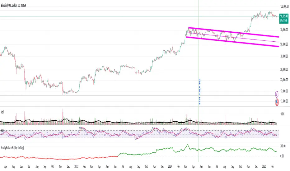
TPO IQ [TradingIQ]Hello Traders!
Introducing "TPO IQ"!
TPO IQ offers a Time Price Opportunity profile with several customization options that packs several related features to help traders navigate the generated profiles!
Features
TPO Profiles
Single Print identification
Initial Balance Identification
Can be anchored to timeframe change
Can be anchored to fixed time interval
Last profile detailed visuals
Customizable value area percentage
POC identification
Mid-point identification
TPO Profiles
A TPO profile is a market profile visualization that details how much time was spent at each price level throughout the time interval.
The image above further explains what a TPO Profile is!
Each letter corresponds to a candlestick. With this information, traders are able to visualize how much time was spent at each price area.
With customizable gradient colors, specifically in this example, blocks colored red are the earliest times in the profile, blocks colored green are in the beginning half of the time midpoint of the profile. Blue blocks represent the first half of the end of the time period, and purple blocks correspond to the end of the time period.
Please note that this form of TPO profile generation will only occur when the most recent profile uses less than 500 alphabet characters! If more than 500 characters are preset, TPO IQ will revert to using labels!
Initial Balance
TPO IQ also identifies the initial balance range and all alphabet characters that form within it!
The image above exemplifies this feature. The initial balance range is denoted by a a neon-blue line, with a blue circle showing the opening price. All characters within the initial balance range are highlighted blue, which is a feature that can be disabled with customizable colors.
POC
TPO IQ also identifies the point of control (POC) of the TPO Profile.
The point of control for the profile is labeled yellow by default, and shows where price spent the most time throughout the time period.
The image above shows the POC for the time period being identified by TPO IQ.
Value Area
TPO IQ also identifies the value area of the profile. A customizable percentage that is 70% by default, the value area of a TPO profile shows where price traded the majority of the time.
The image above further explains this feature. For this example, with the value area percentage being set to 70%, the value area high and value area low show the price zone that prices traded at 70% of the time throughout the profile.
TPO Midpoint
In addition to the POC, the TPO profile midpoint is also identified by TPO IQ.
The TPO midpoint simply corresponds to the middle price between the session's high and low!
Fixed Interval Mode
By default, TPO IQ recalculates every day, but this can also be changed to a customizable session time, such as 4 hours. If 4 hours is selected, then a new TPO profile will be generated every 4 hours.
However, in Fixed Interval mode, a TPO profile will be generated through a user-defined time range, such as 1300-1700.
In the image above, Fixed Interval mode is applied with a time range of 1300-1700 and, consequently, TPO IQ generates a new profile throughout every 1300-1700 time range!
This feature allows traders to specify time ranges of interest to generate TPO profiles for!
TPO Overview Label
The TPO overview label shows key statistics for the TPO profile generated throughout the trading session!
The "TPO Count" statistic shows how many alphabetical letters were generated for the profile, which is an adequate method to determine the session's volatility and price range.
The "Tick Levels" statistic shows how many tick levels were used to create the profile - another method to determine the volatility and price range of the session.
The "Top Letter" statistic shows which letter appears most throughout the profile. In this example, the top letter was "f", which means throughout creation of the profile, the letter "f" appeared the most!
And that's all for now!
If you have any feedback or new feature ideas for TPO IQ please feel free to share them with us!
Thank you traders!

Enhanced Interval Candle with Breakout Detection and Detailed InThis indicator visualizes the last candle of a user-defined time interval (e.g., 1 hour, 4 hours, 1 day) on the current chart, providing enhanced details and breakout detection. It fetches the open, high, low, and close prices of the interval candle and draws a stylized representation of it, offset to the right of the current bar. The candle body and wicks are colored according to whether the interval candle closed bullishly (green) or bearishly (red). In addition to the candle itself, the indicator displays horizontal dotted lines representing the high, low, and midpoint of the interval candle, along with labels showing their exact values. These labels are dynamically updated as the interval candle changes. Furthermore, the script detects and visualizes breakouts of the interval candle's high or low. When the current price closes above the interval high, a green dashed line and a "Bullish Breakout" label are displayed. Conversely, when the current price closes below the interval low, a red dashed line and a "Bearish Breakout" label are shown. The breakout lines and labels are also dynamically updated. This indicator helps traders easily track the price action of a higher timeframe candle and spot potential breakouts based on that candle's range. The user can configure the time interval to suit their trading needs.

Time Based StatisticsThis indicator is a complex time-based statistics tool for analyzing intraday trading patterns. Here's a comprehensive breakdown:
1. **Session Management**
- Tracks trading sessions from 18:00 to 16:59 next day (using New York time)
- Separates analysis by weekdays (Monday through Friday)
- Resets statistics at week's end
2. **High/Low Time Tracking**
- Records when daily highs and lows occur for each day
- Maintains historical arrays of high/low times for pattern analysis
- Tracks high/low patterns in three main time periods:
- Evening/Overnight (18:00-23:59)
- Early Morning (00:00-09:59)
- Market Hours (10:00-16:59)
3. **Probability Calculations**
The indicator calculates several probabilities:
a) **Hold Probability**
- Calculates likelihood current high/low will remain day's high/low
- Counts how many historical highs/lows occurred in remaining hours
- Returns percentage based on historical patterns
b) **Most Frequent Times**
- Identifies which times most frequently produce highs/lows
- Tracks both primary and secondary (next highest) probable times
- Maintains historical counts of highs/lows by hour
4. **Pattern Analysis**
- Filters historical times based on current time
- Helps predict potential future high/low times
- Adjusts analysis based on time of day
5. **Data Display**
Shows statistics in a table including:
- Days of data analyzed
- Current day's high/low times
- Most frequent times for today's highs/lows
- Probability of current high/low holding
- Historical patterns for current hour
6. **Historical Data Management**
- Stores daily high/low data at week's end
- Maintains separate arrays for each day of the week
- Uses this historical data for pattern analysis
The indicator helps traders by:
- Understanding when highs/lows typically occur
- Assessing probability of new highs/lows
- Identifying historically significant time periods
- Providing statistical basis for timing decisions
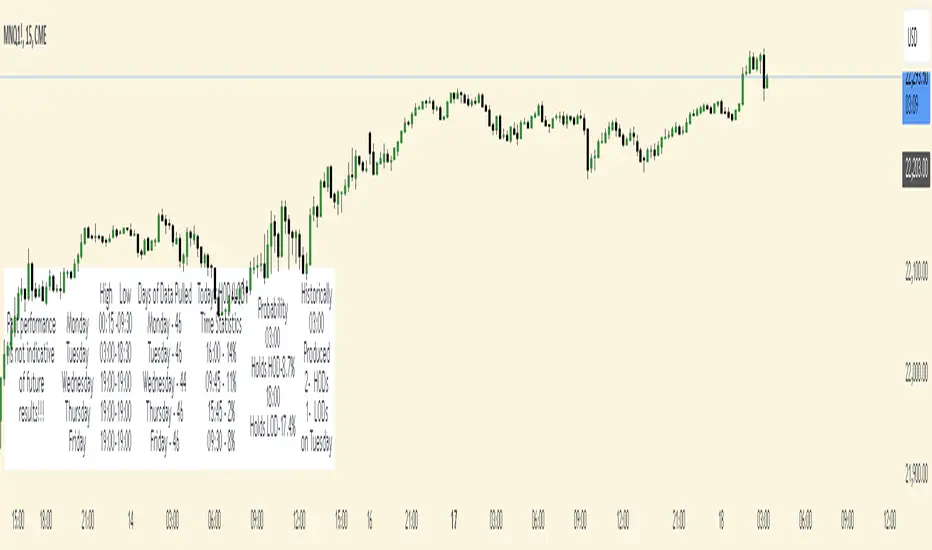
Asset Correlation Heatmap [SeerQuant]Asset Correlation Heatmap
Overview:
The Asset Correlation Heatmap is a powerful visualization tool designed to analyze and compare the correlation between multiple assets and a selected benchmark. The indicator provides a heatmap representation of correlation coefficients, allowing for easy identification of highly correlated and uncorrelated assets at a glance.
How It Works:
Benchmark Asset: The benchmark is the chart that the indicator is applied to. For example, if applied to BTC, the heatmap will display the correlation of various assets relative to BTC.
Correlation Calculation: The script calculates the correlation coefficient between the benchmark asset and each of the 30 user-selected assets over a user-defined period.
Heatmap Display: The results are plotted in a stacked format where the bottom-most plot represents Asset 1, and the top-most plot represents Asset 30.
Each asset’s correlation is color-coded based on its strength (from positive correlation to negative correlation).
Inputs & Customization:
Correlation Length: Users can adjust the lookback period for correlation calculation (default: 20 periods).
30 Selectable Assets: The indicator allows users to input up to 30 assets for correlation analysis.
Color Gradient: The heatmap dynamically assigns colors based on correlation strength where blue shades → strong positive correlation, neutral white → no correlation (~0.0) and red shades → strong negative correlation.
Table Display
A dynamic table in the bottom-right corner provides key insights, including:
Benchmark Asset (the chart symbol)
Highest Correlated Asset & its correlation value
Lowest Correlated Asset & its correlation value
Average & Median Correlation across all selected assets
Composite Signal based on the overall correlation trend
Use Cases
Portfolio Diversification: Identify assets that are highly correlated or negatively correlated with your benchmark to manage risk.
Mean Reversion & Trend Following: Spot assets diverging from their historical correlation to identify trading opportunities.
Pair Trading: Find assets with strong positive or negative correlation to develop hedging strategies.
Enjoy!

Footprint IQ Pro [TradingIQ]Hello Traders!
Introducing "Footprint IQ Pro"!
Footprint IQ Pro is an all-in-one Footprint indicator with several unique features.
Features
Calculated delta at tick level
Calculated delta ratio at tick level
Calculated buy volume at tick level
Calculated sell volume at tick level
Imbalance detection
Stacked imbalance detection
Stacked imbalance alerts
Value area and POC detection
Highest +net delta levels detection
Lowest -net delta levels detection
CVD by tick levels
Customizable values area percentage
The image above thoroughly outlines what each metric in the delta boxes shows!
Metrics In Delta Boxes
"δ:", " δ%:", " ⧎: ", " ◭: ", " ⧩: "
δ Delta (Difference between buy and sell volume)
δ% Delta Ratio (Delta as a percentage of total volume)
⧎ Total Volume At Level (Total volume at the price area)
◭ Total Buy Volume At Level (Total buy volume at the price area)
⧩ Total Sell Volume At Level (total sell volume at the price area)
Each metric comes with a corresponding symbol.
That said, until you become comfortable with the symbol, you can also turn on the descriptive labels setting!
The image above exemplifies the feature.
The image above shows Footprint IQ's full power!
Additionally, traders with an upgraded TradingView plan can make use of the "1-Second" feature Footprint IQ offers!
The image above shows each footprint generated using 1-second volume data. 1-second data is highly granular compared to 1-minute data and, consequently, each footprint is exceptionally more accurate!
Imbalance Detection
Footprint IQ pro is capable of detecting user-defined delta imbalances.
The image above further explains how Footprint IQ detects imbalances!
The imbalance percentage is customizable in the settings, and is set to 70% by default.
Therefore,
When net delta is positive, and the positive net delta constitutes >=70% of the total volume, a buying imbalance will be detected (upwards triangle).
When net delta is negative, and the negative net delta constitutes >=70% of the total volume, a buying imbalance will be detected (downwards triangle).
Stacked Imbalance Detection
In addition to imbalance detection, Footprint IQ Pro can also detect stacked imbalances!
The image above shows Footprint IQ Pro detecting stacked imbalances!
Stacked imbalances occur when consecutive imbalances at sequential price areas occur. Stacked imbalances are generally interpreted as significant price moves that are supported by volume, rather than a significant result with disproportionate effort.
The criteria for stacked imbalance detection (how many imbalances must occur at sequential price areas) is customizable in the settings.
The default value is three. Therefore, when three imbalances occur at sequential price areas, golden triangles will begin to print to show a stacked imbalance.
Additionally, traders can set alerts for when stacked imbalances occur!
Highest +Delta and Highest -Delta Levels
In addition to being a fully-fledged Footprint indicator, Footprint IQ Pro goes one step further by detecting price areas where the greater +Delta and -Delta are!
The image above shows price behavior near highest +Delta price areas detected by Footprint IQ!
These +Delta levels are considered important as there has been strong interest from buyers at these price areas when they are traded at.
It's expected that these levels can function as support points that are supported by volume.
The image above shows a similar function for resistance points!
Blue lines = High +Delta Detected Price Areas
Red lines = High -Delta Detected Price Areas
Value Area Detection
Similar to traditional volume profile, Footprint IQ Pro displays the value area per bar.
Green lines next to each footprint show the value area for the bar. The value area % is customizable in the settings.
CVD Levels
Footprint IQ Pro is capable of storing historical volume delta information to provide CVD measurements at each price area!
The image above exemplifies this feature!
When this feature is enabled, you will see the CVD of each price area, rather than the net delta!
And that's it!
Thank you so much to TradingView for offering the greatest charting platform for everyone to create on!
If you have any feature requests you'd like to see for Footprint IQ, please feel free to share them with us!
Thank you!
